Instruction Pipeline

Instruction Pipeline

• We have seen various cycles involved in the instruction cycle. These fetch, decode and execute cycles for several instructions are performed simultaneously to reduce overall processing time. This process is referred to as instruction pipelining.

• To apply the concept of instruction pipelining, we must subdivide instruction processing in number of stages as given below.

S1 – Fetch (F) : Read instruction from the memory.

S2 – Decode (D) : Decode the opcode and fetch source operand (s) if necessary.

S3 – Execute (E) : Perform the operation specified by the instruction.

S4 – Store (S) : Store the result in the destination.

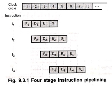
• Here, instruction processing is divided into four stages hence it is known as four–stage instruction pipeline. With this subdivision and assuming equal duration for each stage we can reduce the execution time for 4 instructions from 16 time units to 7 time units. This is illustrated in Fig. 9.3.1.

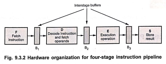
• In this instruction pipelining four instructions are in progress at any given time. This means that four distinct hardware units are needed, as shown in Fig. 9.3.2. These units are implemented such that they are capable of performing their tasks simultaneously and without interfering with one another. Information from the stage is passed to the next stage with the help of buffers.

Example: 1

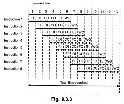
Explain the function of a six segment pipeline and draw a space diagram for a six segment pipeline showing the time it takes to process eight tasks.

Solution :

Six stages in the pipeline :

1) Fetch Instruction (FI) : Read the next expected instruction into a buffer.

2) Decode Instruction (DI) : Determine the opcode and the operand specifiers.

3) Calculate Operands (CO) : Calculate the effective address of each source operand.

4) Fetch Operands (FO) : Fetch each operand from memory.

5) Execute Instruction (EI) : Perform the indicated operation and store the result, if any in the specified destination operand location.

6) Write Operand (WO) : Store the result in memory.

Example: 2

What is the ideal speed–up expected in a pipelined architecture with 'n' stages? Justify your answer.

Solution :

The pipelined processor ideally completes the processing of one instruction in each clock cycle, which means that the rate of instruction processing with n stage pipeline is n times that of sequential operation. Therefore, ideal speed–up factor is n.

However, such ideal performance of the pipeline is achieved only when pipeline stages must complete their processing tasks for a given instruction in the time allotted. Unfortunately, this is not the case; pipeline operations could not sustained without interruption throughout the program execution.

 

1. Pipeline Hazards

• The timing diagram for instruction pipeline operation shown in Fig. 9.3.1 completes the processing of one instruction in each clock cycle. This means that the rate of instruction processing is four times that of sequential operation.

• The potential increase in performance resulting from pipelining is proportional to the number of pipeline stages. However, this increase would be achieved only if pipelined operation shown in Fig. 9.3.1 could be performed without any interruption throughout program execution. Unfortunately, this is not the case.

• For many of reasons, one of the pipeline stages may not be able to complete its wind operation in the allotted time.

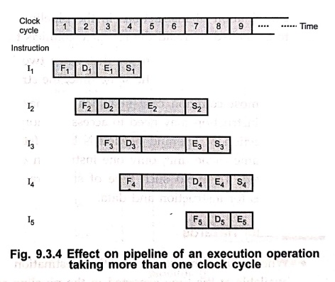
• Fig. 9.3.4 shows an example in which the operation Clock specified in instruction 2 requires three cycles to complete, from cycle 4 through cycle 6. Thus, in 5 and 6, the information in buffer B₂ must remain intact until the instruction execution stage has completed its operation. This means that stage 2 and in turn, stage 1 are blocked from accepting new fort on instructions because the information in B₁ cannot be overwritten. Thus decode step for instruction and fetch step for instruction 5 must be postponed as shown in the Fig. 9.3.4.

• The instruction pipeline shown in Fig. 9.3.4 is said to have been stalled for two clock cycles (clock cycles 5 and 6) and normal pipeline operation resumes in clock 7.

• Any reason that causes the pipeline to stall is called a hazard.

Types of Hazards

1. Structural hazards : These hazards are because of conflicts due to insufficient resources when even with all possible combination, it may not be possible to overlap the operation.

2. Data or data dependent hazards : These result when instruction in the pipeline depends on the result of previous instructions which are still in pipeline and not completed.

3. Instruction or control hazards : They arise while pipelining branch and other instructions that change the contents of program counter. The simplest way to handle these hazards is to stall the pipeline. Stalling of the pipeline allows few instructions to proceed to completion while stopping the execution of those which results in hazards.

 

2. Structural Hazards

• The performance of pipelined processor depends on whether the functional units are pipelined and whether they are multiple execution units to allow all possible combination of instructions in the pipeline. If for some combination, pipeline has to be stalled to avoid the resource conflicts then there is a structural hazard.

• In other words, we can say that when two instructions require the use of a given hardware resource at the same time, the structural hazard occurs.

• The most common case in which this hazard may arise is in access to memory. One instruction may need to access memory for storage of the result while another instruction or operand needed is being fetched. If instructions and data reside in the same cache unit, only one instruction can proceed and the other instruction is delayed. To avoid such type of structural hazards many processors use separate caches for instruction and data.

 

3. Data Hazards

• When either the source or the de When either the source or the destination operands of an instruction are not available at the time expected in the pipeline and as a result pipeline is stalled, we say such a situation is a data hazard.

• Consider a program with two instructions, I₁ followed by I₂. When this program is executed in a pipeline, the execution of these two instructions can be performed concurrently. In such case the result of I₁ may not be available for the execution of I₂. If the result of I₂ is dependent on the result of I₁ we may get incorrect result if both are executed concurrently. For example, assume A = 10 in the following two operations :

I₁    :    A ← A + 5

I₂   :    B← A × 2

• When these two operations are performed in the given order, one after the other, we get result = 30. But if they are performed concurrently, the value of A used in computing B would be the original value, 10, leading to an incorrect result. In this case data used in the I₂ depend on the result of I₁. The hazard due to such situation is called data hazard or data dependent hazard. To avoid incorrect results we have to execute dependent instructions one after the other (in–order).

 

4. Control (Instruction) Hazards

• The purpose of the instruction fetch unit is to supply the execution units with a steady stream of instructions. This stream is interrupted when pipeline stall occurs either due to cache miss or due to branch instruction. Such a situation is known as instruction hazard.

• Instruction hazard can cause greater degradation in performance than data hazards.

1. Unconditional Branching

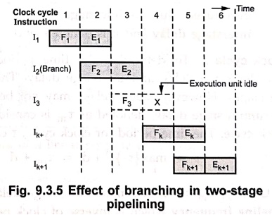
• Fig. 9.3.5 shows a sequence of instructions being executed in a two–stage pipeline. The instruction I₂ is a branch instruction and its target instruction is I_k. In clock cycle 3, the instruction I₃ is fetched and at the same time branch instruction (I₂) is decoded and the target address is computed. In clock cycle 4, the incorrectly fetched instruction I₃ is discarded and instruction I_K is fetched. During this time execution unit is idle and pipeline is stalled for one clock cycle.

Branch Penalty : The time lost as a result of a branch instruction is often referred to as the branch penalty.

Factor effecting branch penalty

1. It is more for complex instructions.

2. For a longer pipeline, branch penalty is more.

In case of longer pipelines, the branch penalty can be reduced by computing the branch address earlier in the pipeline.

 

5. Pipeline Performance

• To measure the performance of pipelined CPU we have to consider the performance measures. A pipeline's performance can be measured by its throughput in terms of millions of instructions executed per second or MIPS.

• Another popular measure of performance is the number of clock cycles per instruction or CPI. These quantities are related by the equation.

CPI = f / MIPS

where f is the pipeline's clock frequency in MHz, and the values of CPI and MIPS are average figures that can be determined experimentally by processing number of representative programs.

• Another general measure of pipeline performance is the speedup S(m) defined by

S(m) = T(1)  / T(m)

where T(m) is the execution time for some target program on an m–stage pipeline and T(1) is the execution time for the same program on a similar, nonpipelined processor.

• Each pipeline stage is a combinational logic circuit. It requires a specific amount of time in terms of propagation delay to process the input data. The precessing time in each stage is known as stage delay. It is denoted as τ. The delays are also introduced due to interstage transfer data. These time delays are known as interstage delay and it is denoted as d.

• Clock cycle : To determine the time period for the clock cycle it is necessary to consider stage delay and interstage delay. The interstage delays can be same between the stages. However, stage delays may not be same for different stages. In such cases, maximum stage delay, denoted as τ_m is considered to determine the time period for the clock cycle. The time period for clock cycle, τ can be given as

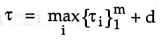
Usually, τ_m >> d and maximum stage delay dominates the clock period. Therefore, pipeline frequency which is inverse of clock period can be given as

f = 1 / τ

Clock skewing : Ideally, we expect the clock pulse to arrive at all stage latches at the same time. In practice, the same clock pulse may arrive at different stages with a time offset of s. This problem is known as clock skewing. The offset s is large for longer logic paths within the stages. Let us denote t_max be the time delay of the longest logic path within a stage and t_min be the time delay of the shortest logic path within a stage. These t_max and t_min put two constraints on the clock period as effect of clock skewing:

τ_m  ≥  t_max +  s       and

d  ≤  t_min  –  s

These two constraints on the clock period avoid a race in two successive stages. In ideal case s = 0, and hence t_max = τ_m and t_min = d.

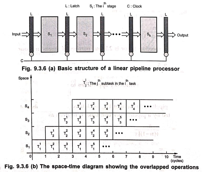
Speedup, efficiency and throughput : Let us consider a space–time diagram in a linear pipeline processor. Fig. 9.3.6 (b) shows the space–time diagram of a four stage pipeline processor. As shown in Fig. 9.3.6 (b), once the pipe is filled up, it outputs one result per clock period independent of the number of stages in the pipe. Ideally, a linear pipeline with m stages can process n tasks in T_m = m + (n − 1) clock cycles, where m cycles are needed to complete the execution of the first task and the remaining n – 1 tasks require n – 1 cycles. Thus the total time required is

T_m = [m + (n − 1)] τ

where t is the clock period.

• The space–time diagram shown in Fig. 9.3.6 (b) has four stages and five tasks. Therefore, the ideal total time required is

T_m = [4 + (5 – 1)] τ

= 8 clock cycles (Refer Fig. 9.3.6 (b))

• The amount of time required to execute same number of tasks in a non–pipeline processor can be given as

T₁ = n mτ

Speedup factor : The speedup factor of a m–stage pipeline over an equivalent non–pipelined processor is defined as

S_m  = T₁ / T_m  = nmτ / [m+(n–1)] τ = nm / m+(n–1)

• For example, if pipeline has four stages and five tasks, its speedup factor is

S₄ = 4×5 / 4+(5–1) = 20 / 8

    = 2.5

• It can be noticed that maximum speedup is S_k →m as n → ∞. However, this maximum speed is very difficult to achieve because of data dependencies between successive task (instructions), program branches, interrupts and other factors, to be studied in subsequent sections.

Efficiency : The efficiency of a linear pipeline is defined as a ratio of speedup factor and the number of stages in the pipeline. The efficiency of m–stage pipeline is given as

E_m = S_m / m = nm /  [ m+(n–1) ] ÷ m

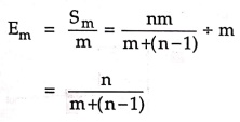
= n /  m+(n–1)

• For example, if speedup factor is 2.5 and number of stages are four, the efficiency can be given as

E_m  = 2.5 / 4 = 0.625

• It can be noticed that the efficiency approaches to unity when

n → ∞, When n = 1, efficiency is minimum. It is 1 / m.

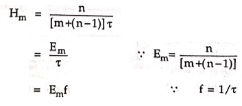
Throughput : The pipeline throughput H_m is defined as the number of results (tasks) that can be completed by a pipeline per unit time. It is given as

H_m = n / [m+(n–1)]τ

= E_m / τ                   E_m= n / [m+(n–1)]

= E_mf                      f = 1 / τ

• In the ideal case, H_m = 1/τ = f when E_m → 1. This means that the maximum throughput of a linear pipeline is equal to its frequency, which corresponds to one output result per clock period. The overall throughput of pipeline is always less than f. This is because usually E_m < 1.

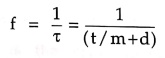
Performance/Cost Ratio (PCR) : Let us consider t be the total time required for a non–pipelined sequential program of a given function. To execute the same program on a m–stage pipeline with an equal flow–through delay t, one needs a clock period of τ = t/m + d, where d is the latch delay. Therefore maximum throughput for m–stage pipeline can be given as

f =  1 / τ    =  1 / (t / m+d)

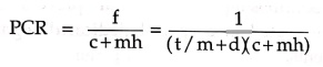
• The total pipeline cost is roughly estimated by c + mh, where c represents cost of all logic stages and h represents the cost of each latch. With this information, in 1973, Larson has defined a pipeline performance/cost ratio as

PCR = f /  c+mh =1 / (t / m+d )(c+mh)

Optimal number of stages :

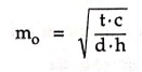
We know that performance of the pipeline can be increased by increasing pipeline stages. Many times pipeline stages are subdivided upto logic gates level called micropipelining to increase parallelism. However, increase in pipeline stages increases the cost of pipelining. Therefore, the optimal choice of the number of pipeline stages should be able to maximize a performance / cost ratio. Fig. 9.3.7 shows the graph of PCR Vs k–stages. The peak of curve corresponds to an optimal choice for the number of desired pipeline stages. It is given as

m₀ =  [ t.c / d.h ]

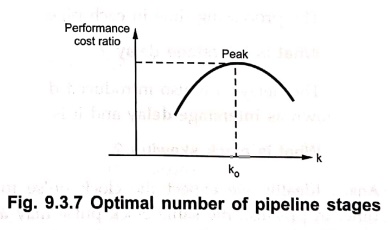
where t is the total flow–through delay of the pipeline, c is the total stage cost, d is the latch delay and h is the latch cost.

 

Review Questions

1. Explain the basic concepts of pipelining.

2. Explain basic operation of a four stage pipelining with a neat diagram.

3. What is instruction pipelining? How it improves performance of computer.

4. Discuss the various hazards that might arise in a pipeline.

5. Explain the issues affecting pipeline performance.

6. Define structural hazard, data hazard and control hazard.

7. Describe in brief any one pipeline hazard.

8. Which are the basic performance issues in pipelining.

9. Define

a. Pipeline frequency

b. Clock skewing

c. Pipeline throughput

d. Speedup factor

e. Pipeline efficiency

f. Performance / cost ratio.