Parallel Processing Challenges

Parallel Processing Challenges

• The tall challenge facing the industry is to create hardware and software that will make it easy to write correct parallel processing programs that will execute efficiently in performance and energy as the number of cores per chip scales.

• It is difficult to write software that uses multiple processors to complete one task faster, and the problem gets worse as the number of processors increases.

• We must get better performance or better energy efficiency from a parallel processing program on a multiprocessor. Lowered

• It is difficult to write parallel processing programs that are fast, especially as the number of processors increases.

• For parallel programming, the challenges include scheduling, partitioning the task into parallel pieces, balancing the load evenly between the processors and so on.

 

1. Amdahl's Law

• Amdahl's law is used to calculate the performance gain that can be obtained by improving some portion of a computer. It states that the performance improvement to be gained from using some faster mode of execution is limited by the fraction of the time the faster mode can be used.

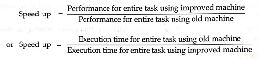
• Speed up (Performance improvement) : It tells us how much faster a task can be executed using the machine with the enhancement as compare to the original machine. It is defined as

Speed up = Performance for entire task using improved machine /  Performance for entire task using old machine

or Speed up = Execution time for entire task using old machine / Execution time for entire task using improved machine

• Fraction enhanced : It is the fraction of the computation time in the original machine that can be converted to take advantage of the enhancement. For example, if CPU's I/O section is enhanced and it is assumed that CPU is busy 60% of the time in I/O operations, then fraction enhanced = 0.6. Fraction enhanced is always less than or equal to 1.

• Speed up _enhanced : It tells how much faster the task would run if the enhancement mode was use for the entire program. For example, if CPU's I/O section is made 10 times faster than Speed up enhanced is 10. Speed up enhancement is always greater than 1.

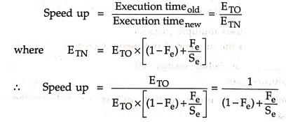
• Amdahl's law gives us a quick way to find the speed up from two factors : fraction enhance (F_e) and speed up enhanced (S_e). It is given as

Speed up = Execution time _old  / Execution time _new  =  E_TO / E_TN

where

E_TN = E_TO × [(1–F_e) + F_e/S_e]

Speed up = E_TO / ( E_TO × [(1– F_e ) + F_e / S_e ) = 1 / ( (1– F_e ) + F_e / S_e)

Example: 1

What percentage of the original computation can be sequential to achieve a speedup of 90 times faster with 100 processors ?

Solution :

Given : Speed up = 90, Speed enhanced = S_e = 100, F_e = ?

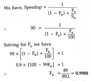
We have, Speedup = 1 / [ (1–F_e) + F_e/S_e ]

90 = 1 / [ (1− F_e) + F_e/100 ]

Solving for Fe we have

90 × [ (1–F_e) + F_e/100 ] = 1

0.9 × [100 – 99F_e] = 1

F_e = 89 / 89.1 = 0.9988

Thus to achieve a speedup of 90 from 100 processors, the sequential percentage can only be 0.11 %.

 

2. Speedup Challenge – Increase in Problem Size

• Getting good speedup on a multiprocessor while keeping the problem size fixed is harder than getting good speedup by increasing the size of the problem. Let us solve the following example to understand this concept.

Example: 2

We have to perform two sums: one is a sum of 20 scalar variables, and one is a matrix sum of a pair of two–dimensional arrays, with dimensions 20 by 20. Let us assume only the matrix sum is parallelizable. What speedup do we get with 10 versus 50 processors? Also calculate the speedups assuming the matrices grow to 40 by 40.

Solution :

Let us assume that single addition can be performed in time t. There are 20 additions that do not benefit from parallel processors and 400 (20 × 20) additions that do. The time required for a single processor to perform all additions will be 420t. The execution time for 10 processors is

Execution time after improvement = Execution time affected by improvement / Amout of improvement + Execution time unaffected

= 400t / 10 + 20t = 60t

So the speedup with 10 processors is 420t/60t = 70

The execution time for 50 processors is

Execution time after improvement = (400t / 50) + 20t = 28t

So the speedup with 50 processors is 420t / 28t = 15

Thus, for this problem size, we get about 70% (7/10 × 100) of the potential speedup with 10 processors. However, we get only 30% (15/50 × 100) speedup with 50 processors.

When we increase matrix (40 × 40) the sequential program now takes

1600t+20t=1620t. The execution time for 10 processors is

Execution time after improvement = (1600t / 10)  20t = 180t

So the speedup with 10 processors is 1620t / 180t = 9

The execution time for 50 processors is

Execution time after improvement =  (1600t / 50) + 20t = 52t

So the speedup with 50 processors is 1620t / 52t = 31.15

Thus, for this larger problem size, we get 90% ( 9 / 10 × 100 ) of the potential speedup with 10 processors and 62.3 % ( 31.15 / 50 × 100 ) with 50 processors.

• The above problem introduces two terms that describe ways to scale up.

■ Strong scaling : Speedup achieved on a multiprocessor without increasing the size of the problem.

■ Weak scaling : Speedup achieved on a multiprocessor while increasing the size of the problem proportionally to the increase in the number of processors.

Example: 3

Suppose you want to perform two sums : one is a sum of 10 scalar variables and one is a matrix sum of a pair of two–dimensional arrays, with dimensions 10 by 10. For now let's assume only the matrix sum is parallelizable ; we'll see soon how to parallelize scalar sums. What speed–up do you get with 10 versus 40 processors? Next, calculate the speed–ups assuming the matrices grow to 20 by 20.

Solution : Let us assume that single addition can be performed in time t. There are 10 additions that do not benefit from parallel processors and 100 (10 × 10) additions that do. The time required for a single processor to perform all additions will be 100t. The execution time for 10 processors is

Execution time after improvement = Execution time affected by improvement / Amout of improvement + Execution time unaffected

= (100 t / 10 )+ 10 t = 20t

So the speedup with 10 processors is 110t/20t = 5.5

The execution time for 40 processors is

Execution time after improvement = (100t / 40 ) +10t = 12.5t

So the speedup with 40 processors is 110t / 12.5t = 8.8

Thus, for this problem size, we get about 55 % (5.5/10 × 100) of the potential speedup with 10 processors. However, we get only 22 % (8.8/40 × 100) speedup with 40 processors.

When we increase matrix (20 × 20) the sequential program now takes

400t+10t = 410t. The execution time for 10 processors is

Execution time after improvement = (400 t / 10) + 10 t = 50t

So the speedup with 10 processors is 410t/50t = 8.2

The execution time for 40 processors is

Execution time after improvement = (400t / 40) + 10 t = 20t

So the speedup with 40 processors is 410t/20t = 20.5

Thus, for this larger problem size, we get 82 % (8.2 / 10) ×100 of the potential speedup with 10 processors and 51.25 % [(20.5 / 40)×100 ] with 40 processors.

Example: 4

Protein String Matching Code has 4 days execution time on current machine doing integer instructions in 20% of time, doing I/O in 35 % of time and other operations in the remaining time. Which is better tradeoff among the following two proposals? First : Compiler optimization that reduces number of integer instructions by 25 % (assume each integer instruction takes the same amount of time); Second : Hardware optimization that reduces the latency of each I/O operations from 6 us to 5 μs.

Solution :

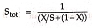
If we can speed up X of the program by S times, Amdahl's law gives the total speed up, S_tot.

S_tot = 1 /  (X/S + (1−X))

First case : Speed integer instruction time,

X = 0.2

S = 1 / (1 – 0.25) = 1.33

S_INT = 1 / [(0.2/1.33) + (1 – 0.2)] = 1.052

Second case : Speedup I/O operation time,

X = 0.35

S = 6 μs / 5 μs = 1.2

S_IO = 1 / [(0.35/1.2)+(1 − 0.35)] = 1.062

Thus, speeding up I/O operations is better.

3 Speedup Challenge – Balancing Load

Example: 5

We have achieved the speedup of 31.15 on the previous bigger problem size with 50 processors. In that problem we assumed the load was perfectly balanced. That is, each of the 50 processors perform 2 % of the work. In this problem we have to calculate the impact on speedup if one processor's load is higher than all the rest. Calculate the impact on speedup if the hardest working processor's load is 4 % and 10%. Also calculate the utilization of the rest of the processors ?

Solution :

a) If one processor has 4 % of the parallel load, then it must do 4 % × 1600 or 64 additions, and the other 49 processors will share the remaining 1536 additions. Since they are operating simultaneously, we can just calculate the execution time as

Execution time after improvement = max ( 1536t / 49 , 64t / 1 ) = 84t

Speedup = 1620 t / 84t = 19.29

The speedup drops from 31.15 to 19.29.

Utilization of remaining 49 processors = 1536t / 49 = 31.35t

Thus we can say that the remaining 49 processors are utilized less than half the time as compared to 64t for hardest working processor.

b) If one processor has 10 % of the load, it must perform 10 %  × 1600 or 160 additions. Thus,

Execution time after improvement = max (1440/49 , 160t / 1) + 20t = 180t

Speedup = 1620 t / 180t  = 9

In this case, the speedup drops to 9.

Utilization of remaining 49 processors  =  1440t / 49  =  29.39 t

Thus we can say that the remaining 49 processors are utilized less than 20 % of the time as compared to 160t for hardest working processor.

• The above example tells the importance of balancing load.

Review Questions

1. Write a note on parallel processing challenges.

2. Explain the Amdahl's law.

3. Justify the following statement with the help of example : "Getting good speedup on a multiprocessor while keeping the problem size fixed is harder than getting good speedup by increasing the size of the problem."

4. What do you mean by strong scaling and weak scaling?

5. Explain the importance of load balancing with the help of suitable example.

6. Explain instruction level parallel processing. State the challenges of parallel processing.

7. Discuss the challenges in parallel processing with necessary examples.

8. Discuss the challenges in parallel processing in enhancing computer architecture.