Vector Processor

Vector Processor

• A vector processor, or array processor, is a CPU design where the instruction set includes operations that can perform mathematical operations on multiple data elements simultaneously. This is in contrast to scalar processor which handles one element at a time using multiple instructions. The vast majority of CPUs are scalar (or close to it). Vector processors were common in the scientific computing area, where they formed the basis of most supercomputers.

• The need to increase computational power is a never ending requirement. In scientific and research areas, the computations involved are quite extensive and hence high power computers are a must.

• The areas like structural engineering, petroleum exploration, aerodynamics, hydrodynamics, nuclear research, tomograph, VLSI design, AI can have data in the form of matrices which suits vector processors to process it at a high speed.

• Some examples of it are :

1. In radar and signal processing for detection of space / underwater targets.

2. In remote sensing for earth resources exploration.

3. In computational wind tunnel experiments.

4. In 3D stop action computer assisted tomography.

5. Weather forecasting.

6. Medical diagnosis.

 

1. Characteristics of Vector Processing

1. A vector is an ordered set of elements. A vector operand contains an ordered set of n elements, where n is called the length of the vector. Each element in a vector is a scalar quantity, which may be floating point number, an integer, a logical value, or a character (byte).

2. In vector processing, two successive pairs of elements are processed each clock period. The dual vector pipes and the dual sets of vector functional units allow two pairs of elements to be processed during the same clock period. As each pair of operations is completed, the results are delivered to appropriate elements of the result register. The operation continues until the number of elements processed is equal to the count specified by the vector length register.

For example :

C(1 : 50) = A(1 : 50) + B(1 : 50)

This vector instruction includes the initial addresses of the two source operands, one destination operand, the length of the vectors and the operation to be performed.

3. Vector instructions are classified into four basic types :

f₁ : V → V

f₂ : V→ S

f₃ : V × V→V

f₄ : V × S → V

where V indicates vector operand and S indicates scalar operand. The operations f₁ and f₂ are unary operations such as vector square root, vector sine, vector complement, vector summation and so on. On the other hand, operations f₃ and f₄ are binary operations such as vector add, vector multiply, vector–scalar add and so on.

4. In vector processing, identical processes are repeatedly invoked many times, each of which can be subdivided into subprocesses.

5. In vector processing, successive operands are fed through the pipeline segments and require as few buffers and local controls as possible. This parallel vector processing allow the generation of more than two results per clock period. The parallel vector operations are automatically initiated either when successive vector instructions use different functional units and different vector registers, or when successive vector instructions use the result stream from one vector register as the operand of another operation using a different functional units. This process is known as chaining.

6. Because of the startup delay in a pipeline, a vector processors perform better with longer vectors.

7. Vector processing is usually faster and more efficient than scalar processing because it reduces the overhead associated with maintenance of the loop–control variables.

 

2. Vector Processing Approach

• In order to reduce the amount of time required to access data from memory, most modern CPUs use a technique known as instruction pipelining in which the instructions pass through several sub–units in turn. The first sub–unit reads the address and decodes it, the next "fetches" the values at those addresses, and the next does the math itself. With pipelining the "trick" is to start decoding the next instruction even before the first has left the CPU, in the fashion of an assembly line so the address decoder is constantly in use. Any particular instruction takes the same amount of time of complete, a time known as the latency, but the CPU can process an entire batch of operations much faster than if it did so one at a time.

• Vector processors take this concept one step further. Instead of pipelining just the instructions, they also pipeline the data itself. They are fed instructions that say not just to add A to B, but to add all of the numbers "in the array A to all of the numbers from array B". Instead of constantly having to decode instructions and then fetch the data needed to complete them, it reads a single instruction from memory and "knows" that the next address will be one larger than the last. This allows for significant savings in decoding time.

• To illustrate what a difference this can make, consider the simple task of adding two groups of 10 numbers together. In a normal programming language you would write a "loop" that picked up each of the pairs of numbers in turn, and then added them. To the CPU, this would look something like this :

Execute this loop 10 times

read the next instruction and decode it

fetch first number

fetch second number

add them

put the result here

end loop

But to vector processor, this task looks considerably different :

read instruction and decode it

fetch 10 numbers

fetch 10 numbers

add them

put the results here

• There are several savings inherent in this approach. For one, only two address translations are needed. Depending on the architecture, this can represent a significant savings by itself. Another savings is fetching and decoding the instruction itself, which only has to be done one time instead of ten. The code itself is also smaller, which can lead to more efficient memory use.

• But more than that, the vector processor typically has some form of superscalar implementation, meaning there is not one part of the CPU adding up those 10 for numbers, but perhaps two or four of them. Since the output of a vector command are does not rely on the input from any other, those two (for instance) parts can each add five of the numbers, thereby completing the whole operation in half the time. This is parallel processing approach for vector computation.

• In the above discussion we have seen the vector computation approach. Let us see the processor organization that can be used to implement vector computation approach. The processor organizations used for vector computation can be categorized as :

■ Pipelined ALU

■ Parallel ALU

■ Parallel Processors

Pipelined ALU

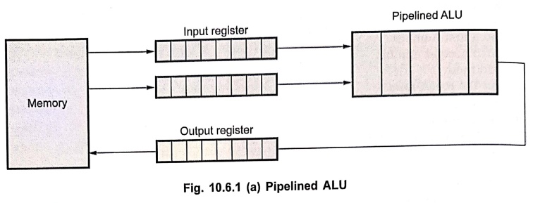
• Fig. 10.6.1 (a) shows the pipelined ALU organization. The complex ALU operations such as floating point operations are decomposed into stages. These stages can be pipelined using pipelined ALU. A pipelined ALU will save time only if it is fed a stream of data from sequential locations. A single, isolated floating point operation is not speeded up by a pipeline. The speedup is achieved when a vector of operands is presented to the ALU,

parallel ALU

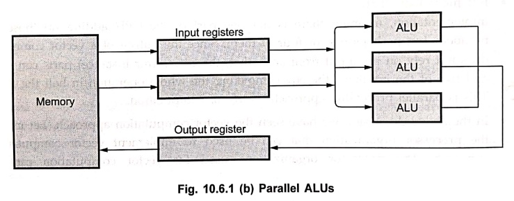
• Fig. 10.6.1 (b) shows the parallel ALU organization. Here, multiple ALUs in a single processor are used to implement vector processing approach. In this case, the control unit of the processor routes data to ALUs so that they can function in parallel. It is also possible to use pipelining on each of the parallel ALUs to further speedup the operation.

Parallel processors

In the parallel processor organization, the multiple ALUs from multiple processors operate in parallel. The ALUs sometimes called processing units (PE) are synchronized to perform the same function at the same time. Such processors are also known as array processors. In short, an array processor is a synchronous parallel computer with multiple ALUS. The array processor can handle single instruction and multiple data streams. Because of this reason, array processors are also known as SIMD processors.

Example: 1

Define vector and vector instruction format. Also explain matrix multiplication with the help of inner product calculation on a pipeline processor.

 Solution :

A vector is an ordered set of one–dimensional array of data items. It is represented as a row vector by V = (V1 V2 V3 ... Vn] where V is a vector and n is a length of a vector. It may be represented as a column vector if the data items are listed in a column. A computer capable of vector processing allows operations to be specified with a single vector instruction as follows

C(1 : 100) = A(1 : 100) + B(1 : 100)

This vector instruction adds two vectors A and B of length 100 to produce a vector C.

Fig. 10.6.2 shows the instruction format of vector instruction. It is a three–address instruction. It includes operation code, the base addresses of the source operands, the base address of the destination operand, and the length of the vectors all in one composite instruction.

Inner product is one of the most popular operations performed in computers with vector processors. The inner product consists of the sum of k product terms of the form

C = A₁B₁ + A₂B₂ + A₃B₃ +……… + A_kB_k

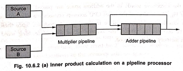
Fig. 10.6.2 (a) shows the inner product calculation on a pipeline processor, Here, the values of A and B vectors are either in memory or in processor registers. A four–segment floating point multiplier and four–segment floating point adder pipelines are used. A_i and B_i pairs are brought in and multiplied at a rate of one pair per cycle. Assuming that k = 100, after the first four cycles, the products begin to be added to the output of the adder (initially cleared). The first addition will take place in the ninth cycle is A₁ B₁ + A₅ B₅. The tenth cycle starts the addition A₂B₂ + A₆B₆ and so on. This pattern breaks on the summation into four sections as follows :

C = A₁B₁ + A₅ B₅ + A₉B₉ + ... + A₉₇B₉₇

A₂B₂ + A₆B₆ + A₁₀B₁₀ + …+ A₉₈B₉₈

A₃B₃ +A₇B₇+ A₁₁B₁₁+ ... + A₉₉B₉₉

A₄B₄+ A₈B₈ + A₁₂B₁₂ + ... + A₁₀₀B₁₀₀

The adder pipeline will then have one partial product in each of its four segments. The four partial sums must then be added in an additional step to form the final sum.

Matrix multiplications is one of the most computational intensive operations within which the inner product is used. Let us consider the 3 × 3 matrices A and B.

The product matrix C is a 3 × 3 matrix whose elements can be determined by the inner product as,

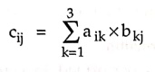
For example, C₁₁ can be calculated as,

C₁₁ = a₁₁ b₁₁ + a₁₂b₂₁ + a₁₃b₃₁

Each element is determined by three multiplications and three additions (if C_ij is initialized to 0). Thus the total number of multiplications or additions required to compute the matrix product is 9 × 3 = 27, i.e. n³ where two matrices are n × n. The multiplication of two n × n matrices requires 9 (n²) inner products.

 

3. Memory Interleaving

• Pipeline and vector processors often require simultaneous access to memory from two or more sources. An instruction pipeline may require the fetching of opcode and operand at the same time from two different memory segments. Similarly, arithmetic pipeline may require two or more operands to enter the pipeline at the same time. In such systems, the memory access time is the bottleneck and one way to reduce it is to use cache memory. 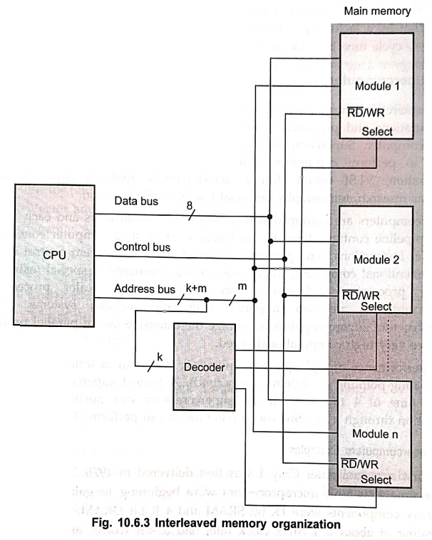Alternative technique to reduce memory access time is memory interleaving. In this technique, the main memory is divided into a number of memory modules and the addresses are arranged such that the successive words in the address space are placed in different modules. Refer Fig. 10.6.3. Most of the times CPU accesses consecutive memory locations. In such situations, addresses will be to the different modules. Since these modules can be accessed in parallel, the average access time of fetching word from the main memory can be reduced.

• The low–order k bits of the memory address are generally used to select a module, and the high–order m bits are used to access a particular location within the selected module. In this way, consecutive addresses are located in successive modules. Thus, any component of the system that generates requests for access to consecutive memory locations can keep several modules busy at any one time. This results in both faster access to a block of data and higher average utilization of the memory system as a whole. It is important to note that to implement the interleaved memory structure, there must be 2^k modules; otherwise, there will be gaps of nonexistent locations in the memory address space.

• The effect of interleaving is substantial. However, it does not speed up memory operation by a factor equal to the number of the module. It reduces the effective memory cycle time by a factor close to the number of modules.

 

4. Supercomputers

• A commercial computer with a capacity of performing large–scale vector or matrix computations and pipelined floating–point arithmetic operations is referred to as supercomputer. Supercomputers are very powerful, high–performance computers used to perform computations in areas of structural engineering, petroleum exploration, VLSI circuit design, aerodynamics, hydrodynamics, meteorology, nuclear research, tomography, artificial intelligence and so on.

• Supercomputers are equipped with multiple functional units and each unit has its own pipeline configuration. The instruction set of supercomputer consists of data transfer instructions, data processing instructions and program control instructions of conventional computers. In addition to this it consists of special instructions for vector processing and combination of vector and scalar processing. The supercomputers are also supported with large memory systems. With such infrastructure supercomputers encourage the extensive use of parallel processing to achieve very high computational speed.

• The performance of high–speed computers is evaluated in terms of Flops (number of floating–pointing operations per second). A typical supercomputer has a basic cycle time of 4 to 20 ns. If the supercomputer can calculate a floating–point operation through a pipeline each cycle time, it can perform 50 to 250 megaflops.

1. Supercomputers Examples

• The first supercomputer Cray 1 was first delivered in 1976. This was around the same time that 8–bit microprocessors were beginning to gain popularity, typical memory components were 1K bit SRAM and 4 K bit DRAM. Most machines were operating at about a 1 MHz clock rate, had 32–bit words, and large mainframes had 1 MB to 8 MB of RAM. Cray 1 is a vector machine, with 8 "vector registers" (a vector register is 64 words, each word is 64 bits). It allows us to multiply or  add(subtract) one vector register by another vector register giving a third vector register.

• The Cray 1 consists of –

■ 64–bit words

■ 8 MB of RAM

■ 16–way interleaving on low–order bits

■ 50 ns memory cycle

■ 12.5 ns clock cycle (80 MHz) to achieve the speed of 160 million floating point operations per second (160 megaflops)

■ 12 pipelined functional units

■ The Cray 1 has 3 basic data types : addresses (24–bit integer), integers (64–bit), floating point (64–bit, 48–bit mantissa).

■ The Cray 1 has 12 functional units. These are divided into four groups :

•  Group 1 – Vector units

■ Vector (integer) Add : 3 stages

■ Vector Logical : 2 stages

■ Vector Shift : 4 stages

•  Group 2 – Vector and scalar units

■ Floating Add : 6 stages

■ Floating Multiply : 7 stages

■ Floating Reciprocal Approximation : 14 stages

•  Group 3 Scalar units

■ Integer Add : 3 stages

■ Logical : 1 stage

■ Shift : 2 stages

■ Scalar population count and leading zero count : 3 stages

•  Group 4 – Address units

■ Add : 2 stages

■ Multiply : 6 stages

• Cray 1 instructions are 32 or 16 bits, so from 2 to 4 instructions can be packed into a word. Instructions are thus addressed on 16–bit boundaries while data is addressed on 64–bit boundaries.

• It has 8 megabyte (1 million word) main memory. The memory is divided into 16 banks, with each bank having a 50 ns access time. Therefore, when 16 memory banks are accessed simultaneously, the memory data transfer rate is 320 million words per second.

• Another group within the same company developed the first multiprocessor Supercomputer, the Cray X–MP, which was introduced in 1982. Its cycle time is 9.5 ns. it has mainly added a multiport memory system and increased memory to 16 M words, 32–way interleave. In 1988, Cray Research introduced the Cray Y–MP, the world's first supercomputer to sustain over 1 gigaflop on many applications. Its cycle time is reduced to 6 ns. The Cray–2 system appeared in 1985, providing a tenfold increase in performance over the Cray–1. Its effective cycle time is 8.2 ns. It can access up to 256 M words of memory 64 or 128 way interleave depending on configuration.

2. Practical Considerations in Supercomputer Design

• To achieve such high speeds, high–power (i.e. hot) drivers are employed, signals are detected with specialized analog circuits, conductors are all shielded and precisely tuned in both impedance and length, and data is encoded with error–correcting so that losses can be recovered.

• In addition, the circuits are usually designed to operate in balanced mode so that there is no change in power drawn as drivers switch. As one driver switches from low to high, another switches from high to low, so that the power supply sees a DC load and there is no coupling of switching noise back into the logic via the power supply. In addition, using balanced signal lines can increase the signal to noise ratio by 6 dB, although these are not often used. In a design such as the Cray–1, roughly 40% of the transistors supposedly do nothing but balance the power loading.

• Even so, these machines dissipate large amounts of heat. For the dissipation of heat they use special thermal conduction modules in which a multichip substrate is mounted in a carrier with built–in plumbing for a chilled water jacket.

 

Review Questions

1. Explain the need of vector processing

2. Explain the characteristics of vector processing.

3. Explain vector operation.

4. Explain the general instruction format of the vector processor.

5. Write a short note on memory interleaving.

6. Write a short note on supercomputers.

7. Explain the practical considerations in supercomputer design.

8. Explain vector processing.

9. Explain i) Vector processing ii) Vector operations. Explain how matrix multiplication is carried out on a computer supporting vector computations.