Particle in a one dimensional potential box (infinite potential well)

PARTICLE IN A ONE DIMENSIONAL POTENTIAL BOX (INFINITE POTENTIAL WELL)

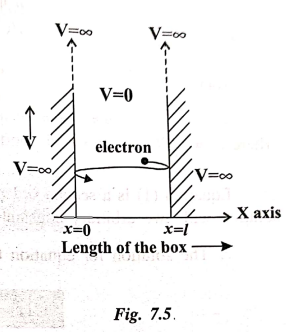
Let us consider a particle (electron) of mass 'm' moving along x‒axis, enclosed in a one dimensional potential box (infinite potential well) as shown in Fig. 7.5.

Since the walls are of infinite potential, the particle does not penetrate out from the

box.

Also, the particle is confined between the length ‘l’ of the box and has elastic collisions with the walls. Therefore, the potential energy of the electron inside the box is constant and can be taken as zero for simplicity.

∴ We can say that Outside the box and on the wall of the box, the potential energy V of the electron is ∞.

Inside the box the potential energy (V) of the electron is zero.

In other words, we can write the boundary conditions as

 V(x)=0 when 0<x<l

 V(x) = ∞ when 0≥x≥l

Since the particle cannot exist outside the box the wave function ᴪ=0 when 0≥x≥l.

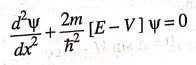
To find the wave function of the particle within the box of length 'l', let us consider the schroedinger one dimensional time independent wave equation (i.e.,)

Since the potential energy inside the box is zero [(i.e) V=0], the particle has kinetic energy alone and thus it is named as a free particle (or) free electron.

∴ For a free particle (electron), the Schroedinger wave equation is given by

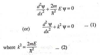
Equation (1) is a second order differential equation, therefore, it should have solution with two arbitrary constants.

∴ The solution for equation (1) is given by

 ᴪ(x) = A sin kx + B cos kx                ………….(3)

where A and B are called as arbitrary constants, which can be found by applying the boundary conditions.

(i.e.,) V(x)  = ∞ when x=0 and x=l

Boundary condition (i) at x=0, potential energy V=∞,  ∴ There is no chance for finding the particle at the walls of the box, .∴ ᴪ(x) = 0

 ∴ Equation (3) becomes

 0 = A sin 0 + B cos 0

 0 = 0 + B(1)

∴ B=0

Boundary condition (ii) at x=1, potential energy V=∞, ∴ There is no chance for finding the particle at the walls of the box, ∴ ᴪ(x) = 0

∴ Equation (3) becomes

 0 = A sin kl + B cos kl

Since B=0 (from 1st Boundary condition), we have

0 = A sin kl

Since A ≠ 0; sin kl = 0

We know sin nπ = 0

Comparing these two equations, we can write kl=nπ

where n is an integer.

(or) k = nπ / l           …………….(4)

Substituting the value of B and k in equation (3) we can write the wave function associated with the free electron confined in a one dimensional box as

 ᴪ_n(x) = A sin (nπx/l)                 ……………..(5)

Energy of the particle (Electron)

We know from equation (2)

Equating equation (6) and equation (7), we can write

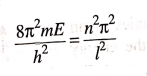
Energy of the particle (electron) E_n = n²h² / 8ml²         …………..(8)

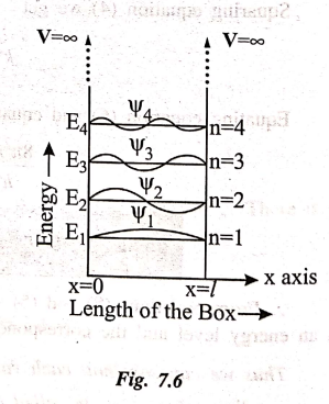
∴ From equations (8) and (5) we can say that, for each value of 'n', there is an energy level and the corresponding wave function.

Thus we can say that, each value of E_n is known as Eigen value and the corresponding value of ᴪ_n is called as Eigen function.

Energy levels of an electron

For various values of 'n' we get various energy values of the electron. The lowest energy value (or) ground state energy value can be got by substituting n=1 in equation (8)

∴ When n=1 we get E₁= h² / 8ml²

Similarly we can get the other energy values

(i.e.,) When n=2 we get E₂= 4h² / 8ml²  ⇒ 4E₁

(i.e.,) When n=3 we get E₃= 9h² / 8ml²  ⇒ 9E₁

(i.e.,) When n=4 we get E₄= 16h² / 8ml²  ⇒ 16E₁

∴ In general, we can write the energy eigen function as

 E_n= n²E₁                ………………..(9)

It is found from the energy levels E₁, E₂, E₃ etc, the energy levels of an electron are Discrete.

This is the great success which is achieved in quantum mechanics than classical mechanics, in which the energy levels are found to be continuous.

The various energy eigen values and their corresponding eigen functions of an electron enclosed in a one dimensional box is as shown in Fig. 7.6. Thus, we have discrete energy values.

Note: The number of nodes and antinodes in the wave with respect to the quantum number can be got from a general formula (ie.,) if we have n number of antinodes then (n+1) number of nodes will be there.

For example if n=3 then ᴪ₃ has 3 antinodes and 4 nodes

(at x=0, x =l/3, x =2l/3 and x=l)

Normalisation of the wave function

Normalisation: It is the process by which the probability (P) of finding the particle (electron) inside the box can be done.

We know that the total probability (P) is equal to 1 means, then there is a particle inside the box.

∴ For a one dimensional potential box of length 'l', the probability

 P = ₀∫¹ |ᴪ|² dx = 1 (Since the particle is present inside the well between the length 0 to’l’ the limits are chosen between 0 to l )        ……..(10)

Substituting equation (5) in equation (10), we get

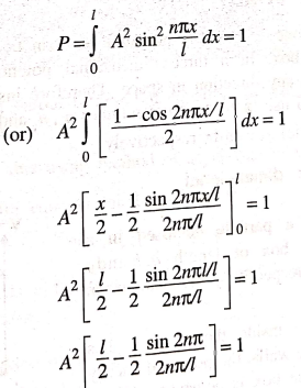
         ...(11)

We know sin nπ = 0

sin 2nπ is also = 0

∴ Equation (11) can be written as

A²l / 2 = 1

(or) A² = 2/l

(or) A = √[2/l]

Substituting the value of 'A' in equation (5),

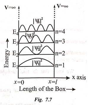
The normalised wave function can be written as

The normalised wave function and their energy values are as shown in Fig. 7.7.