Particle in a three dimensional (3d) Potential box

PARTICLE IN A THREE DIMENSIONAL (3D) POTENTIAL BOX

The solution of one‒dimensional potential box can be extended for a three dimensional potential box. In a three dimensional potential box, the particle (electron) can move in any direction in space. Therefore instead of one quantum number 'n', we have to use three quantum number n_x, n_y, and n_z corresponding the three co‒ordinate axis (ie) x, y and z respectively.

Particle in a three dimensional potential box

Let us consider a particle enclosed in a 3‒dimensional potential box of length a, b and c along x, y and z axis respectively as shown in Fig. 7.8.

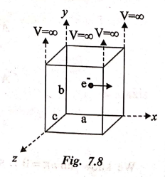
Since the particle inside the 3D box has elastic collisions with the walls, the potential energy of the electron inside the box is constant and can be taken as zero for simplicity.

∴ We can say that outside the box and on the wall of the box, the potential energy is ∞.

 ∴ The boundary conditions are

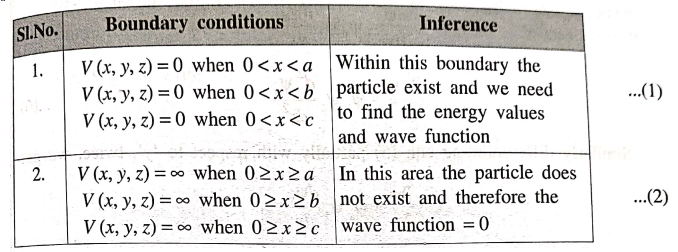
Boundary conditions

1. V (x, y, z) = 0 when 0<x<a

V (x, y, z) = 0 when 0<x<b

V (x, y, z) = 0 when 0 < x <c

Inference: Within this boundary the particle exist and we need to find the energy values and wave function                  ...(1)

2. V (x, y, z) = ∞ when 0≥x≥a

V (x, y, z) = ∞ when 0≥x≥b

V (x, y, z) = ∞ when 0≥ x ≥ c

Inference: In this area the particle does not exist and therefore the wave function = 0          ...(2)

To find the wavefunction of the particle within the boundary conditions (1).

Let us consider the 3‒dimensional schrodinger time independent wave equation,

i.e.,

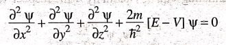
……….....(3)

Since V=0 [For a free particle], we can write eqn (3) as

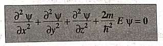
………….. (4)

Equation (4) is a partial differential equation, in which ᴪ is a function of three variables, x, y and z.

∴ We can solve this using method of separation of variables.

∴ The solution for eqn (4) can be written as

 ᴪ(x, y, z) = ᴪ_x ᴪ_y ᴪ_z

Which means ᴪ is a function of x, y and z and is equal to product of 3 functions i.e., ᴪ_x, ᴪ_y, and ᴪ_z.

Where

ᴪ_x is a function of x only

ᴪ_y is a function of y only

ᴪ_z is a function of z only

∴ We can write the solution for equation (4) as ᴪ= ᴪ_x ᴪ_y ᴪ_z                   ………(5)

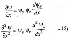
Differentiating eqn (5), Partially with respect to 'x', twice, we get

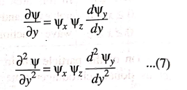
Similarly differentiating eqn (5) partially with respect to 'y', twice, we get

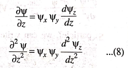
Similarly differentiating eqn (5) partially with respect to 'z', twice, we get

Substituting equations (5), (6), (7) and (8) in eqn (4) we get

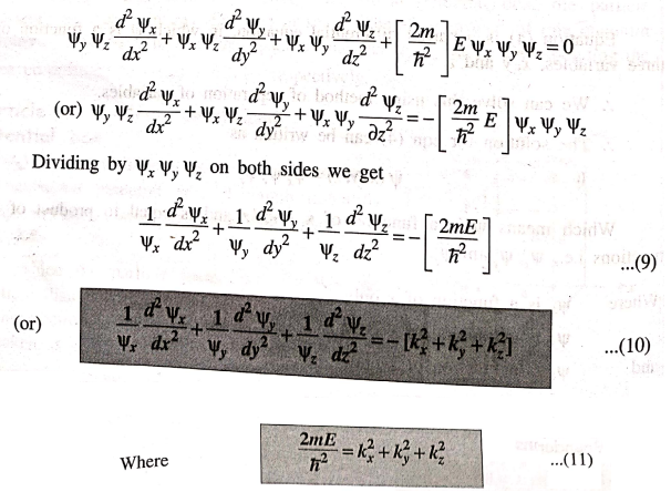
In equation (10), L.H.S. is independent of each other and is equal to a constant in R.H.S. ∴ we can equate each term of L.H.S. to each constant in R.H.S.

∴ We can write

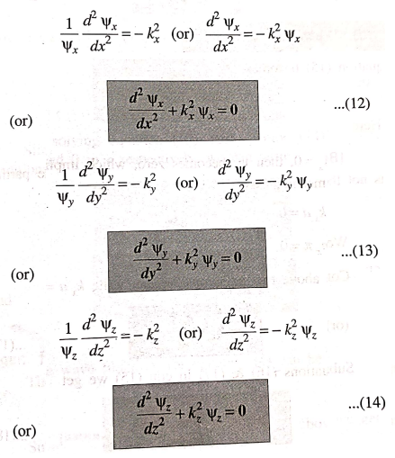
Equations (12), (13) and (14) represents the differential equations in x, y and z co‒ordinates. The solution for equation (12) can be written as

 ᴪ_x = A_x sin k_xx + B_x cos k_xx                …....(15)

where A_x and B_x are arbitrary constants, which can be found by applying boundary conditions.

Boundary Conditions

(i) When x=0; x=0

∴ Equation (15) becomes

 0 = 0 + B_x

∴ B_x = 0                ……...(16)

(ii) When x=a; X=0

∴ Equation (15) becomes

 0=A_x sin k_xa

Here  A_x ≠ 0

 [Because, if А_x=0, then ᴪ_x becomes zero, which implies that the particle is not there, and is meaningless]

∴ sin k_xa = 0

We know sin n_xπ = 0

Comparing the above two equations we can write k_xa = n_xπ

 (or) k_x = n_xπ / a              …………..(17)

Substituting equations (16) & (17) in eqn (15) we get

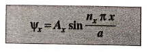
……....(18)

Equation (18) represents the un‒normalized wave function.

Normalization

Eqn (18) can be normalized by integrating it within the limits i.e., boundary conditions 0 to a,

We can write ₀∫^a |ᴪ_x|² dx = 1

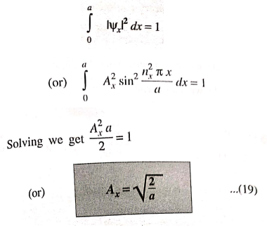
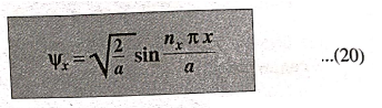
Substituting eqn (19) in (18) we get

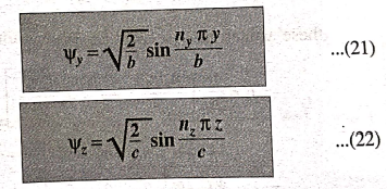
Similarly by solving equation (13) and equation (14) with the boundary conditions 0 to b and 0 to c respectively, we can write

Eigen functions

The complete wave function, for equation (4) can be written as

 ᴪ(x, y, z) = ᴪ_x ᴪ_y ᴪ_z

Substituting equations (20), (21) and (22) in the above equation, we get

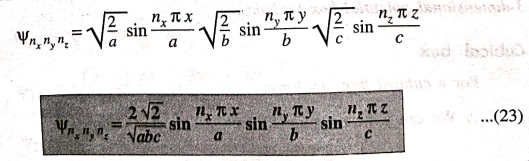
Equation (23) represents the eigen function for an electron in a 3‒dimensional potential box.

Eigen values

From equation (11) we can write

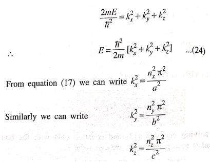
Substituting these values in eqn (24), we get

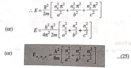
Equation (25) represents the energy eigen values of an electron in a 3‒dimensional potential box (cuboid).

Cubical box

For a cubical box, a = b = c,

∴ We can write equation (25) as

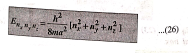
The corresponding normalized wave function of an electron in a cubical box can be obtained from equation (23), as

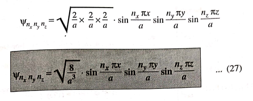
From equations (26) and (27) we can note that, several combinations of the three quantum numbers (n_x, n_y and n_z) leads to different energy eigen values and eigen functions.

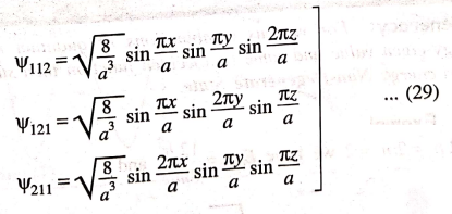
Example

If a state has quantum numbers n_x = 1; n_y = 1; n_z=2

Then, n_x²+n_y²+n_z²= 6

Similarly for n_x=1; n_y=2; n_z=1 combination and n_x=2 , n_y=1 , n_z=1 combination we have n_x²+n_y²+n_z²= 6

E₁₁₂‒E₁₂₁ = E₂₁₁  = 6h² / 8ma²           ………………(28)

The corresponding wave functions can be written as

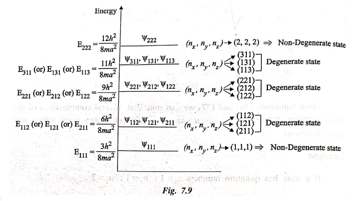
The energy values for various set of quantum number combination is as shown in Fig. 7.9, from which we can conclude that the energy values are discrete.