Change of variables in double integrals

 

CHANGE OF VARIABLES IN DOUBLE INTEGRALS

 

Sometimes, the evaluation of a double integral may become simpler by change of variables. The change of variables may be from

✓ Cartesian to Cartesian coordinates.

✓ Cartesian to Polar coordinates.

 

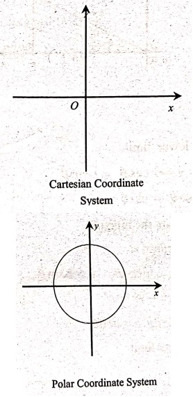
CARTESIAN COORDINATES INTO POLAR COORDINATES

 

Sometimes, the evaluation of a double integral may become simpler by change of variables. Changing from Cartesian coordinates to polar coordinates. i.e., Changing from (x, y) to (r, θ), the variables are related by

x= r cos θ

y= r sin θ

x² + y² = r²

dxdy = |J| drdθ = r drdθ

Note: Whenever ∫∫ f(x, y)dxdy is evaluated throughout the area of a circle, upper half of a circle, quadrant of a circle, it is advantageous to use polar coordinates.

 

Example 59. Change into polar coordinates, ₀∫¹₀∫^x f(x, y) dydx.

Solution:

The polar form is

 x = r cos θ, y = r sin 0

 x² + y² = r²

dxdy = r drdθ

Inner upper limit is

y = x ⇒ r sin θ = r cos θ

 sin θ = cos θ

 tan θ = 1; θ = π/4

 θ varies from θ = 0 to θ = π/4

Outer upper limit x = 1

 r cos 0 = 1

⇒ r = 1 / cosθ

 r varies from r = 0 to r = 1/cosθ

 

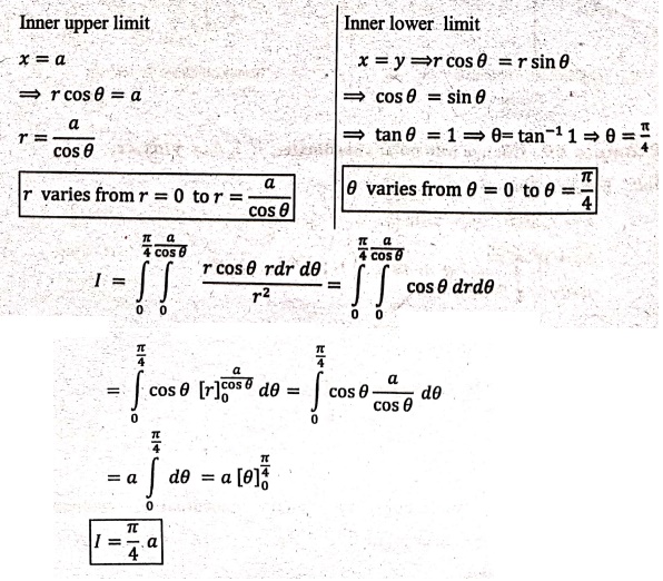
Example 60. By changing to polar coordinates evaluate ₀∫^a_y∫^a ( x / x²+y² ) dxdy.

Solution:

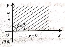
To plot the region

The region of integration is bounded by x=y,

x = a, y = 0, y = a.

To evaluate the integral:

The polar form is

x = r cos θ, y = r sin θ

x² + y² = r²

dxdy = r drdθ

 

Example 61. Evaluate by changing to polar coordinate the integral .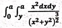

Solution:

To plot the region:

The region of integration is bounded by x = y, x = a, y = 0, y = a.

The polar form is

x = r cos θ, y = r sin θ

x² + y² = r², dxdy = r drdθ

To evaluate the area:

 

Example 62. By converting to polar coordinates evaluate = ₀∫^∞₀∫^∞ e^‒(x2+y2) dxdy, hence find ₀∫^∞e^‒x2 dx.

Solution:

To plot the region:

The region is bounded by x = 0, x = ∞, y = 0, y = ∞

To evaluate the integration:

The polar form is

x = r cos θ, y = r sin θ

x² + y² = r²

dxdy = r drdθ

Since both the lower limits are 0 and region is entire first quadrant,

 θ varies from θ = 0 to θ = π/2

Both the upper limits are ∞,

 r varies from r = 0 to r = ∞

 

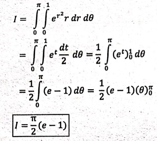
Example 63. Using polar coordinates, evaluate ∫∫_R e^x2+y2 dy dx, where R is the semicircular region bounded by the x‒axis and the curve y = √[1 ‒ x²].

Solution:

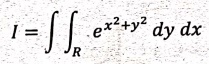
To plot the region:

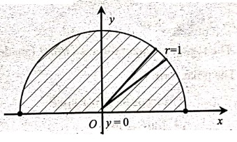
The region R is the semicircular region bounded by x‒axis (y = 0) and the circle x² + y² = 1.

The polar form is

x = r cosθ, y = r sinθ

x² + y² = r², dydx = r drdθ

To find the limit:

Given, x² + y² = 1

⇒ r² = 1

⇒ r = 1

 r varies from r = 0 to r = 1

Region is in first and second quadrant,

 θ varies from θ=0 to θ = π

Put r² = t

2r dr = dt

r dr = dt/2

When r = 0 ⇒ t = 0

When r = 1⇒ t=1

 

Example 64. Change into polar coordinates, dydx and evaluate.

Solution:

To plot the region:

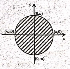
The region is bounded by x = ‒a, x = a

‚y = −√[a² ‒ x²], y = √[a² ‒ x² ]

ie., x²+ y² = a²

The region of integration is OABO (shaded region)

The polar form is

x=rcosθ, y = r sinθ

x² + y² = r²

dxdy = r drdθ

Inner upper limit is y = √[a²‒x²]

i.e.,x² + y² = a²

 r² = a² ⇒ r = a

 r varies from r = 0 tor = a

Since both the lower limits are negative, the region is entire circle x² + y² = a²

 θ varies from θ = 0 to 2π

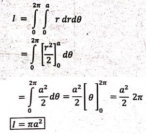
I = πα²

 

Example 65. By Converting into polar co‒ordinates evaluate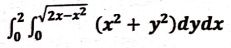 

Solution:

To plot the region:

Since inner limit is a function of x, first integrate with respect to y, then x

The region of integration is bounded by

y = 0, y = √[2x‒x²] i.e. x² + y² ‒ 2x = 0, x = 0, x = 2.

x = 0 is y‒axis

x² + y² ‒ 2x = 0 is a circle with center (1,0) and radius = 1

x = 0 is y‒axis, x = 2 is a straight line perpendicular to x‒axis

To evaluate the integral:

The polar form is

 x = r cosθ, y = r sinθ

x² + y² = r²

dxdy = r drdθ

x² − 2x+1 + y² = 1

i.e. (x‒1)²+ y² = 1²

center (1,0) and radius 1

Since the region is a semi circle lies in first quadrant,

 θ varies from θ=0 to θ=π/2

y= √[2x‒x²]

⇒ y² = 2x − x²

⇒ x² + y² − 2x = 0

r² ‒ 2r cosθ = 0

 r(r ‒ 2cosθ) = 0

  r = 0 or r = 2 cosθ

varies from r = 0 to r = 2 cosθ

 I = 3π / 4

 

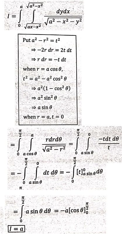
Example 66. Transform the double the double integral in polar coordinates 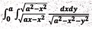 and then evaluate it.

Solution:

The limit of the inner integral containing x term, first integrate with respect to y then x.

To plot the region:

The region of integration is bounded by y = √[ax ‒ x²], y = √[a² − x²],

x = 0, x = a.

i.e.,x²+y²‒ax = 0 & x² + y² = a²

x² + y² ‒ ax = 0

⇒ (x – a/2)² + (y − 0)² = (a/2)²

i.e., the circle with centre at (a/2,0) and radius a/2

 x²+y² = a² is a circle with centre (0,0) and radius a.

The region of integration is between the two circles which lies in the first quadrant.

To evaluate the integral:

The polar form is

x = r cosθ, y = r sinθ

x² + y² = r²

dxdy = r drdθ

Since the region lies in first quadrant which touches both x and y axes,

 θ varies from θ = 0 to θ = π/2

x² + y² − ax = 0 ⇒ r² ‒ ar cosθ = 0

r(r ‒ a cosθ) = 0

r = 0 or r = a cosθ

Take r = a cosθ

x² + y² = a² ⇒ r² = a² ⇒ r = a

 r varies from r = a cosθ tor = a

 

 

EXERCISE

 

43. Using polar coordinates, evaluate ∫∫_R e^(x2+y2) dydx, where R is the semi-circular region bounded by the x‒axis and the curve y = √[1‒x²]. Ans: π/2 (e‒1)

 

44. Evaluate the following by changing to polar coordinates

 

45. Evaluate 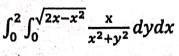 by changing to polar coordinates. Ans: π/2

 

46. Express ₀∫^∞₀∫^∞ f(x, y) dxdy in polar co‒ordinates. Ans: ₀∫^π/2₀∫^∞ f(r, θ)r drdθ.

 

47. Express ₀∫^a_y∫^a  (x²dxdy) / (√[x²+y²]) in polar co‒ordinates and then evaluates it. Ans: a³/3 log(√2 + 1)

 

48. Evaluate ∫∫ (x+y) / (x²+y²+a²) dxdy over the portion of the first quadrant lying inside the circle x² + y² = a². Ans: 2a (1 ‒ π/4)

 

49. Evaluate ∫∫ xy dxdy over the positive quadrant of the circle x² + y² = 1. Ans: 1/8.

 

50. Evaluate ∫∫ √[a²‒x²‒y²] dx dy over the semi‒circle x²+ y² = ax in the positive quadrant. Ans: [a³(3π‒4) ] / 18

 

51. Evaluate ∫∫ (x + y) dx dy over the region in the positive quadrant bounded by the circle x² ‒ 2ax + y² = 0. Ans: (3π‒4)a³ / 48

 

52. Evaluate _‒a∫^a₀∫^√(a2‒x2)  (x²+ y²) dxdy, using polar co‒ordinates. Ans: πa⁴ / 4

 

53. Evaluate ∫∫ √ [ (1‒x²‒y²) / (1+x²+y² )] dx dy over the positive quadrant of the circle x²+ y²

1. Ans: π/2 ( π/4 ‒ 1/2)

 

54. Evaluate ∫∫ sin π(x² + y²)dxdy over the region bounded by the circle x² + y² = 1. Ans: 2

 

55. Evaluate ∫∫ (x²y² ) / (x²+y²) dxdy by changing into polar coordinates over annular region between the circles x²+y² = 16 and x² + y² = 4. Ans: I = 15π

 

56. Transform the integral into the polar coordinates and hence evaluate ₀∫^a₀∫^√[a2‒x2] √[x² + y²] dydx. Ans:  πa³ / 6

 

57. Transforming to polar co‒ordinates, evaluate the integral ₀∫^a₀∫^√[a2‒x2] (x²y+ y³) dxdy. Ans: a⁵ / 5