Regression

Regression

•  When two variables are correlated, we often want to predict one variable using the other. For example ‒ Can we predict a student's marks based on hours studied.

• The process of finding a mathematical relationship between variables is called regression analysis.

• Definition : Regression is statistical method used to describe and predict the relationship between two quantitative variables.

• During regression analysis following are some key terms that are used commonly

■ Dependent Variable(Y) : This is a variable that we want to predict. This is basically an output.

■ Independent Variable(X): This is a variable that is used to predict the dependent variable. This is basically input.

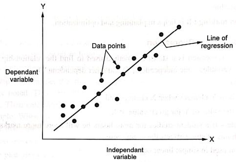
■ Regression Line : It is a straight line that best fits the data points and shows the trend.

Importance of Regression

1. Prediction: The regression technique is used for forecasting future outcome. For Jolly instance ‒ Regression is used to predict the sales or price growth.

2. Trend analysis: Regression is used to understand direction and rate of change.

3. Feature relationship: It is used to quantify how change in one variable affect the other variable.

4. Decision making: It is helps in planning and optimization.

1. Simple Linear Regression

• Simple linear regression is a statistical method used to find the relationship between two quantitative variables ‒ one independent(X) and other dependent(Y). Ushnaqed

• It helps us to ‒

i) Predict how Y changes when X changes and

ii) Predict the value of Y for given value of X.

• For example ‒ If a student studies for more hours he will score more marks. That means number of hours of study affects the exam score.

• The equation used in simple linear equation is of

Y = a + bx

Where

Y is dependent variable(the one we want to predict)

X independent variable(the one we use for prediction)

a intercept(i.e. value of Y when X = 0)

b slope(change in Y for one unit change in X). The slope (b) of a regression line tells us how much the dependent variable (Y) is expected to change for a one‒unit change in the independent variable (X).

Example

If,

Y = 30+5X

That means ‒

When X = 0, minimum 30 will be scored. Here 30 will be intercept.

For every 1 extra hours of study, marks will be increased by 5. Here 5 will be slope.

2. Regression Line

• A regression line is a line of best fit that shows the trend of data points in a scatter plot.

•  It passes through the data such that the total error (difference between actual and predicted values) is minimal.

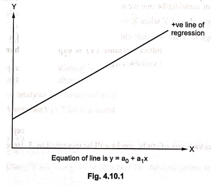
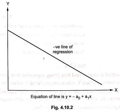
• The line can be upward sloping (positive relation) or downward sloping (negative relation).

1) Positive linear relationship: If the dependent variable increases on the Y‒axis and independent variable increases on X‒axis, then such a relationship is termed as a positive linear relationship.

2) Negative linear relationship: If the dependent variable decreases on the Y‒axis and the independent variable increases on X‒axis, then such a relationship is termed as a negative linear relationship.

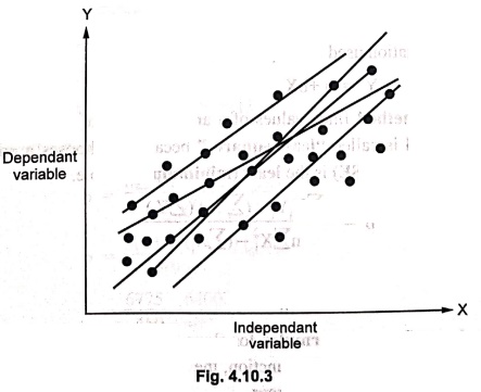
best fit line

While working with linear regression, we need to find the best fit line. This is the line which yields the minimized error between predicted values and actual values. That means the best fit line will have the least error.

Concept of Residual: A residual is the difference between the actual value of Y and the predicted value of Y () obtained from the regression line.com

In symbols:

Residual = Y‒

Residuals help us evaluate how well the regression line fits the data.

Residual tells us how far off our prediction is from the actual value.

• If residual = 0 means perfect prediction (point lies on the regression line)

• If residual > 0 means actual value is above the regression line

•  If residual < 0 means actual value is below the regression line

 

3. Least Squares Regression Line

•  The least square method is used to find best fitting regression line. It minimizes the sum of squared differences between actual Y values and predicted Y values on the line.

•  The Least Squares Regression Line is the straight line that minimizes the sum of the squares of the residuals, where each residual means the difference between the actual value of Y and the predicted value of Y () from the line.

• The formula used is –

minimizes Σ (Y ‒  Y ˆ)²

 where:

• Y = Actual observed value

•  (Y‒hat) = Predicted value from regression line

As we know, the equation used in simple linear equation is

Y = a + bX

• The Least squares method finds values of a and b that make this total error as small as possible. The method is called "least squares" because it chooses a and b such that the Sum of Squared Errors (SSE) is the least (minimum) possible.

b = [ nΣΧ_iΥ_i ‒ (ΣΧ_i) (ΣΥ_i) ] / [ nΣx_i² ‒ (Σx_i)² ]

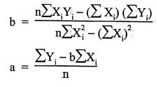
a = [ ΣΥ_i ‒ bΣΧ_i ] /  n

• These are the Least Squares Formulas for slope and intercept. When we substitute these values of a and b back into the SSE function, the SSE is the smallest possible value. Any other pair of a, b will make the SSE larger

Demo Example

Consider the following Student database in which we have number of hours student studied and actual marks obtained.

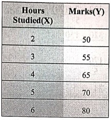
We want to find a relationship so that we can predict marks (Y) from hours studied (X).

Step 1: We will calculate required values

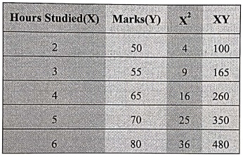
Σx = 20

ΣΥ = 320

ΣX_i²; = 90, ΣX_iY_i = 1355

Step 2: Calculate the slope(b)

b = [ n(ΣXY) – (ΣX) (ΣY) ] /   [nΣX² ‒ (ΣX)²]

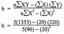
b = [ 5(1355) ‒ (20) (320) ] / [ 5(90) ‒ (20) ]

= 6775‒6400 / 450‒400

= 375/50

Slope(b) = 7.5

Step 3: Calculate the intercept(a)

a = [ ΣY‒b(ΣX) ] / n

a = [320‒7.5(20)] / 5

   = 320‒150 / 5

   = 170/5

a = 34

Intercept (a = 34):

When study hours = 0, the expected marks = 34 (baseline performance).

Slope (b = 7.5):

For each extra hour studied, marks increase by 7.5 points.

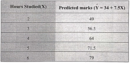
Step 4: Prediction using Regression equation

The predicted marks are close to the actual marks.

Step 5: We will compute squared residual and then sum of squared residual for a= 34 and b = 7.5

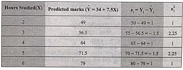
Now, sum of the squared residual SSE(34,7.5) = 1 + 2.25 + 1 + 2.25 + 1 = 7.5

SSE at (34, 7.5) = 7.5

Step 6: Check if it actually gives least squared regression line or not

We have already computed SSE at (34,7.5) = 7.5 for a = 34 and b = 7.5

Now for checking if it gives best fit regression line or not we slightly change the values of a and b.

Case A: Change intercept by +1.

That means a = 35, b = 7.5

 Prediction  = 35+ 7.5X

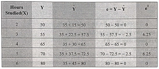
SSE(35, 7.5) = 0 +6.25 +0 +6.25 +0 = 12.5

This is bigger than 7.5.

Case B: Change intercept by ‒ 1.

a = 33, b = 7.5

Prediction  = 33 +7.5X:

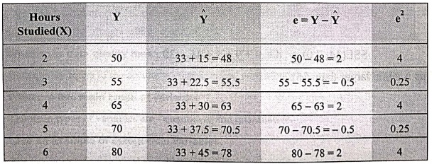
SSE(33, 7.5) = 4+0.25 +4 +0.25 + 4 = 12.5

This again bigger than 7.5.

Case C: Change slope by + 0.5

So, a = 34 and b = 8.0

Prediction  = 34 +8X:

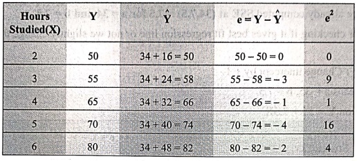
SSE(34, 8) = 0+9+1+16+4=30

This is again very much larger than 7.5

Case D : Change slope by ‒ 0.5

So a = 34, b = 7.0

Prediction  = 34+ 7X :

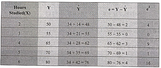
SSE(34, 7.0) = 4+0+9+1+16=30

This is again larger than 7.5

The least square regression line can be represented by following graph

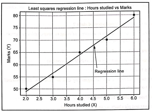
Conclusion:

Small changes to either a or b produce larger SSE (Examples above: 12.5 or 30). This shows that SSE at the least‒squares solution (a,b)=(34,7.5) is 7.5.

 

Review Question

1. Why is the least squares method used in regression analysis?