Derivative of a function

DERIVATIVE AS A FUNCTION

 

In geometry, the tangent line (or simply tangent) to a plane curve at a given point is the straight line that "just touches" the curve at that point. In other words, a tangent line should have the same direction as the curve at the point of contact. As it passes though the point where the tangent line and the curve meet, called the point of tangency, the tangent line is "going in the same direction" as the curve, and is thus the best straight‒line approximation to the curve at that point.

The geometrical idea of the tangent line as the limit of secant lines serves as the motivation for analytical methods that are used to find the tangent lines explicitly. The question of finding the tangent line to a graph, or the tangent line problem, was one of the central questions leading to the development of calculus.

 

The Tangent Problem

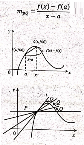
If a curve C has the equation y = f(x) and we want to find the tangent line to C at the point P(a, f(a)), then we consider a nearby point Q(x, f(x)), where x ≠ a, and compute the slope of the secant line PQ:

m_PQ  = [ f(x) ‒ f(a) ] / (x‒a)

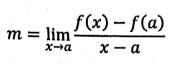
Then we let Q approach P along the curve C by letting x approaches a. If m_PQ approaches a number m, then we define the tangent t to be the line through P with slope m. (This amounts to saying that the tangent line is the limiting position of the secant line PQ as Q approaches P).

 

Definition 1:

The tangent line to the curve y = f(x) at the point P(a, f(a)) is the line through P with slope

provided that this limit exists.

 

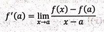
Definition 2:

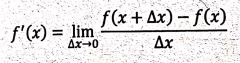
The derivative of a function f at a number a, denoted by f'(a), is

if this limit exists.

If we write x = a + h, then we have h = x‒a and h approaches 0 if and only if x approaches a. Therefore an equivalent way of starting the definition of the derivative, as we saw in finding tangent lines, is

Remark:

The tangent line to y = f(x) to (a, f(a)) whose slope is equal to f'(a), the derivative of f at a. Using point‒slope form, the tangent line can be expressed as

 y‒f(a) = f'(a)(x − a)

 

Definition 3:

A function f is differentiable at a if f'(a) exists. It is differentiable on an open interval (a, b) [or (a, ∞) or (‒∞, a) or (‒∞, ∞)] if it is differentiable at every number in the interval.

 

Definition 4:

The tangent line x = a to y = f(x) is said to be a horizontal tangent if f'(a) = 0.

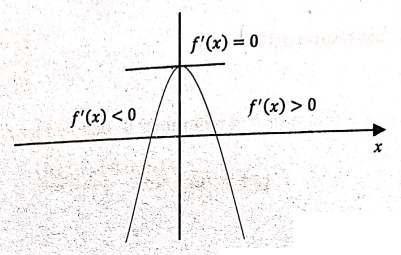
Derivatives can help graph many functions. The first derivative of a function is the slope of the tangent line for any point on the function. Therefore, it tells when the function is increasing, decreasing or where it has a horizontal tangent. Consider the following graph. Notice on the left side, the function is increasing and the slope of the tangent line is positive. At the vertex point of the parabola, the tangent is a horizontal line, meaning f '(x)= 0 and on the right side the graph is decreasing and the slope of the tangent line is negative.

 

 

1. THE PRODUCT, QUOTIENT AND CHAIN RULES

The product rules

Theorem: If ƒ and g are both differentiable, then

Proof: Let u = f(x) and v = g(x) are both positive differentiable functions. Then x changes by an amount Δx, then the corresponding changes in u and v are

Δu = f(x + Δx) ‒ f(x), Δv = g(x + Δx) ‒ g(x)

Δ(uv) = (u + Δu)(v + Δv) ‒ uv

= uΔv + vΔu + ΔuΔv

If we divide by Δx, we get

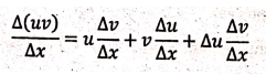
If we now let Δx→ 0, we get the derivative of uv:

 

The Quotient Rule:

Theorem: If ƒ and g are both differentiable, then

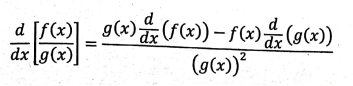
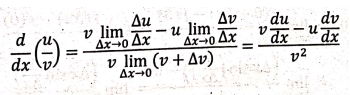
Proof:

We find a rule for differentiating the quotient of two differentiable functions u = f(x) and v = g(x) in much the same way that we found the Product Rule. If x, u and v change by amount Δx, Δu, and Δv, then the corresponding change in the quotient u/v is

As Δx → 0, Δv→ 0 also, because v = g(x) is differentiable and therefore continuous. Then, using the Limit Laws, we get

 

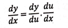
Chain Rule:

If g is differentiable at x and ƒ is differentiable at g(x), then the composite function f = fog defined by F(x) = f(g(x)) is differentiable at x and F' is given by the product

F '(x) = f '(g(x)). g'(x)

In Leibniz notation, if y = f(u) and u = g(x) are both differentiable functions, then

dy/dx =  dy/du • du/dx

Proof: Let Δu (Δu ≠ 0) be the change in u corresponding to a change of Δx in x, that is, Δu = g(x + Δx) − g(x).

 

 

PROBLEMS UNDER DERIVATIVES

Let y = f(x) be a function defined on R. Then

Derivate at a point x = a is f '(a) =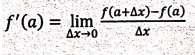 

 

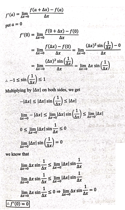
Example 91. Determine whether f '(0) exist or not f(x) =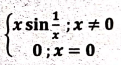 

Solution:

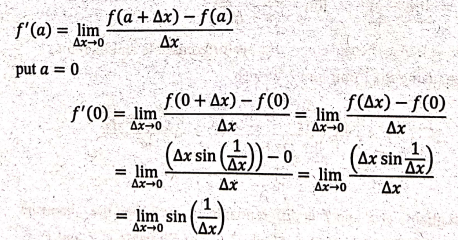
This value is not unique (value lies between ‒1 and 1)

 f '(0) does not exists.

 

Example 92. Determine whether f'(0) exist or not f(x) = 

Solution:

 

Example 93. Whether is the function f(x) = |x| is differentiable?

Solution:

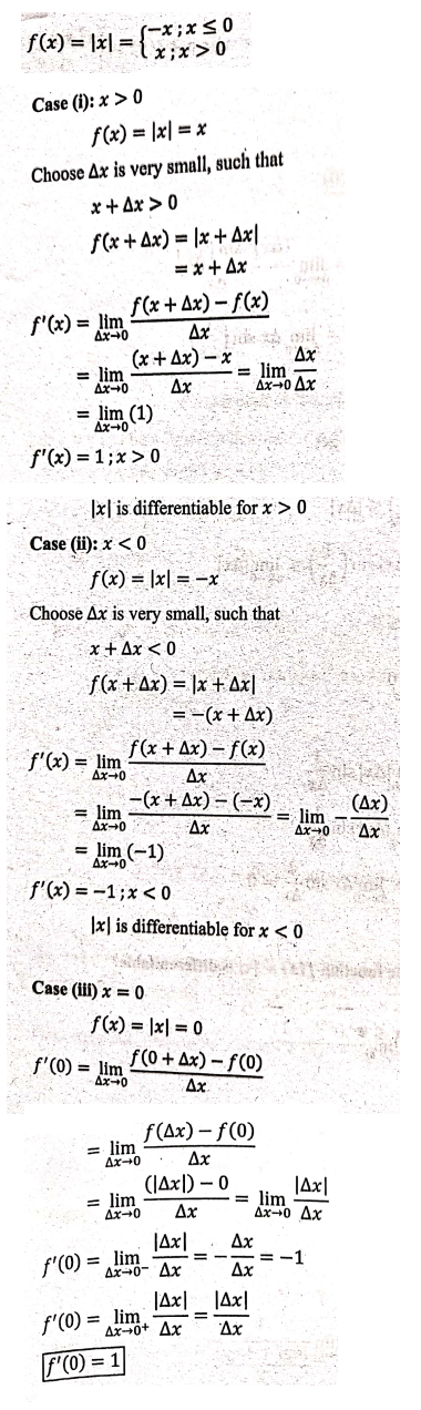
 f '(0) = 1

Since f '(0) is not unique, f '(0) dose not exits.

Hence f(x) = |x| is differentiable expect at the origin.

Both continuity and differentiability are desirable properties for a function. The following theorem shows how these properties are related.

Theorem: Every differentiable function is continuous

Remark: Continuous function need not be differentiable.

Example: f(x) = |x| is continuous at origin but not differentiable at origin.

 

 

2. DIFFERENTIATION OF SOME STANDARD FUNCTIONS

 

Example 94. Find the derivative of constant function.

Solution: Let f(x) = c

:. f(x + Δx) = c

f '(x) = 0

 

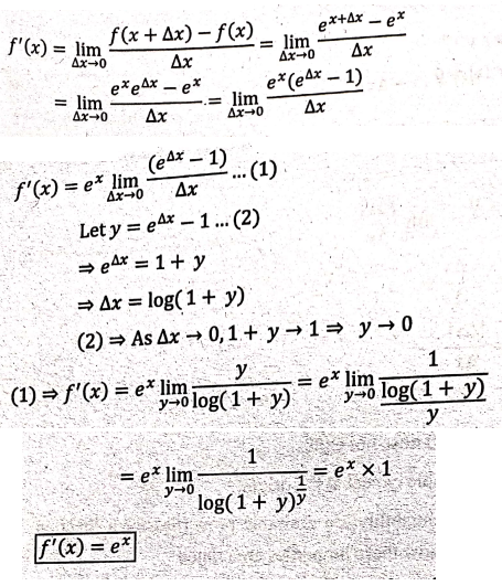
Example 95. Find the derivative of the function f(x) = e^x.

Solution: Let f(x) = e^x

 f(x + Δx) = e^x+Δx

 

Example 96. Find the derivative of the function f(x) = log x

Solution:

 

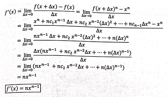
Example 97. Find the derivative of the function f(x) = xⁿ; n is a positive integers.

Solution: Let f(x) = xⁿ

:. f(x+Δx) = (x + Δx)ⁿ

 

 

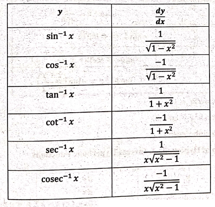
3. DIFFERENTIATION OF INVERSE TRIGONOMETRIC FUNCTIONS

 

 

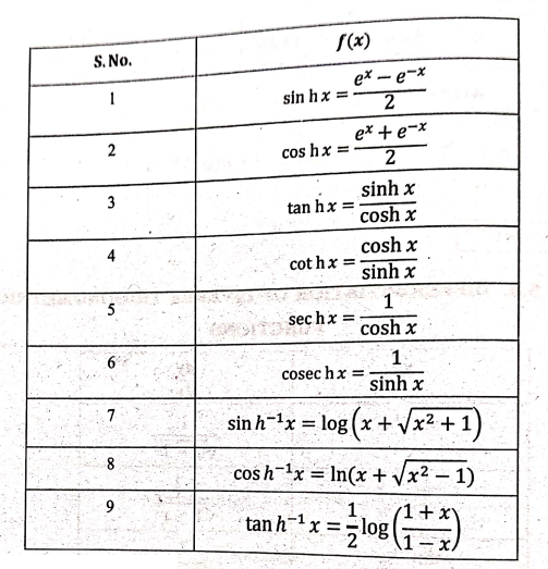
4. DERIVATIVES OF HYPERBOLIC FUNCTIONS

Some even and odd combinations of the exponential function e^x and e^‒x arise frequently in Mathematics and its applications that they deserve to be given special names. In many ways they are analogous to the trigonometric functions and they have the same relationship to the hyperbola, that the trigonometric functions have to the circle. For this, they are called hyperbolic functions and individually called hyperbolic sine, hyperbolic cosine and so on.

 

Formulae for Hyperbolic & Inverse Hyperbolic Functions

10. cos h²x ‒ sin h²x = 1

11. cos h²x + sin h²x = cos h2x

12. sinh 2x = 2 sinh x cosh x

 

Differentiation of Hyperbolic & Inverse Hyperbolic Functions

 

 

5. PROBLEMS UNDER DERIVATIVES

 

 

Example 98. Find the derivative of (i) x e^‒2x (ii) x(x² ‒ 1)(x²+4)

Solution:

(i) d/dx (xe^‒2x) = x(‒2 e^‒2x) + (1)e^‒2x

= ‒2xe^‒2x + e^‒2x = e^−2x(‒2x+1)

(ii) d/dx [x(x² ‒ 1) (x² + 4)]

= 1(x²‒1)(x²+4) + x(2x)(x²+4) + x(x²‒1)2x

= x² + 4x² ‒ x² ‒ 4 + 2x² + 8x² + 2x² ‒ 2x²

= 5x⁴ +9x² ‒ 4

 

 

Example 110. The equation of motion of a particle is S = 2t³ ‒ 5t² + 3t + 4, where S is measured in centimeters and t in seconds. Find the acceleration as a function of time. What is the acceleration after 2 seconds?

Solution:

It is given that S = 2t³‒5t²+3t+4

Velocity = V(t) = ds/ dt = 6t²‒10t+3

Acceleration = a(t) = dV/ dt = d²s/dt² = 12t‒10

The acceleration after 2 second is a(2) = 24‒10 = 14 cm/sec²

 

 

PROBLEMS UNDER n^th DERIVATIVE OF A FUNCTION

 

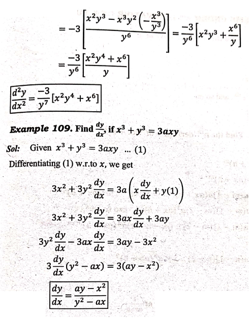
Example 111. Find the n^th derivative of e^ax

Solution:

Let y = e^ax

Then

y' = ae^ax

y" = a²e^ax and so on ...

:: yⁿ = aⁿ e^ax

 

Example 112. Find the n^th derivative of (ax + b)^m.

Solution:

Let y = (ax + b)^m

Then

y' = ma(ax + b)^m‒1

y" = ma(m − 1)a(ax + b)^m‒2 = m(m−1)a²(ax+b)^m‒2

y"' = m(m − 1)(m − 2)a³(ax + b)^m‒3 and so on....

y⁽ⁿ⁾ = m(m −1)(m − 2) ... (m − n + 1)aⁿ (ax + b)^m‒n

When m = n

y⁽ⁿ⁾ = n(n − 1)(n − 2) ... 1 × aⁿ (ax + b)°

 .. y⁽ⁿ⁾ = n! aⁿ

 

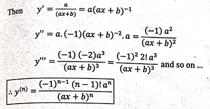
Example 113. Find the nth derivative of 1 / ax+b

Solution:

 

Example 114. Find the n^th derivative of log(ax + b)

Solution:

Let y = log(ax + b)

 

Example 115. Find the n^th derivative of sin(ax + b)

Solution:

Let y=sin(ax + b)

Then

y' = acos(ax+b)

= asin (ax+b+π/2)

= asin(ax + b')            where b' = b + π/2

y" = a² cos(ax + b')

 = a² sin (ax + b' + π/2) = a² sin (ax + b + π/2 + π/2)

= a² sin (ax+b+2(π/2))

y''' = a³sin (ax+b+3(π/2)) and so on...

 y⁽ⁿ⁾ = aⁿ sin (ax + b + n(π/2) )

 

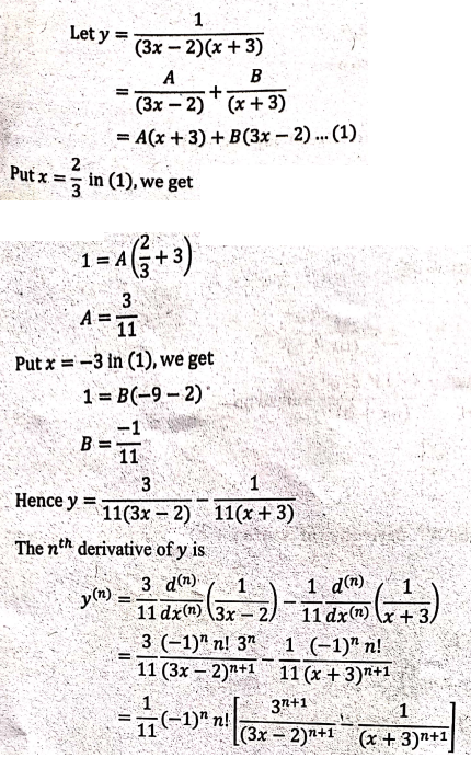
Example 116. Find the n^th differential coefficient of 1 / [(3x‒2)(x+3)] with respect to x.

Solution:

 

Example 117. If f(x) = xe^x then find f'(x). Also find the n^th derivative fⁿ(x).

Solution:

Let f(x) = xe^x

To find f '(x)

Then f '(x) = xe^x + e^x          (1)

 f '(x) = xe^x + e^x

To find the n^th derivative

 f "(x) = xe^x + e^x(1) + e^x

= xe^x + 2e^x

ƒ'''(x) = xe^x + e^x(1) + 2e^x

= xe^x + 3e^x and so on...

: f ⁿ(x) = xe^x + ne^x

fⁿ(x) = (x + n)e^x

 

 

6. DERIVATIVES USING LOGARITHM

 

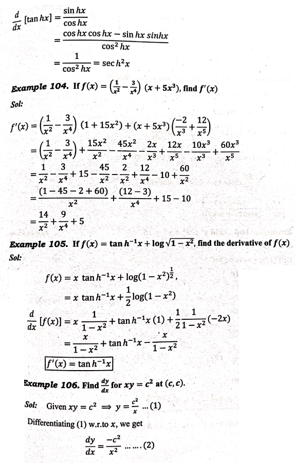
Example 118. Find the differential coefficient of 

Solution:

 

Example 119. If y = a^x, find dy/dx.

Solution:

y = a^x

log y = log a^x

log y = xloga^x

Different w.r.t x

1/y . dy/dx = log a

dy/dx = y loga

dy/dx = = a^x loga

 

Example 120. If y^x = x^y, find dy/dx.

Solution:

 y^x = x^y

log y^x = log x^y

xlog y = y log x

Different w.r.t x

 

Example 121. If y = (sin x)^x, find dy/dx.

Solution:

 y = (sin x)^x

log y = log(sinx)^x

log y = xlog(sin x)

Different w.r.t x

dy/dx = y(x cotx + log sinx)

 

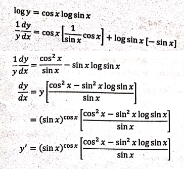
Example 122. Find y' if y = (sin x)^{cos x}

Solution:

Given y (sin x)^{cos x}

log y = cos x log sin x

 

Example 123. If y = u+v where u = x^x, v = x^1/x then find dy/dx.

Solution:

 y = u+v

 

 

 

EXERCISE

 

27. Write the composite function in the form f[g(x)]. [Identify the inner function u = g(x) and the other function y = f(u)]. Then find the derivative

(a) y = sin 4x          Ans: y'(x) = 4 cos 4x

(b) y = (1‒x²)¹⁰          Ans: y'(x) = ‒20x(1 − x²)⁹

(c) y = e^√x          Ans: y' (x) = e^√x / 2√x

 

28. Find the derivative of the functions.

(a) f(x) = ⁴√[1+ 2x + x³]         Ans: f'(x) = 2+3x² / 4(1+2x+x³)^3/4

(b) f(x) = 1 / (x⁴ +1)³         Ans: f '(x) = ‒ [ 12x³ / (x⁴+1)⁴ ]

(c) y(x) = cos(a³ + x³)         Ans: y'(x) = ‒3x² sin(a³ + x³)

(d) f(x) = (2x − 3)⁴(x² + x + 1)⁵         Ans: f '(x) = (2x − 3)³ (x² + x + 1)⁴ (28x² ‒ 12x‒7)

(e) y(x) = [ (x²+1)/(x²+1) ]³              Ans: y'(x) = ‒12x(x²+1)² / (x²‒1)⁴

(f) y(x) = √[1 + 2e^3x]              Ans: y'(x): = 3e^3x / √[1+2e^3x]

(g) F(t) = e^{tsin 2t}              Ans: F ' (t) e^t sin 2t (2t cos 2t + sin 2t)

(h) y(x))=sin(tan 2x)              Ans: y'(x) = 2 cos(tan 2x) sec²(2x)

(i) y(x) = cos ( 1‒e^2x / 1+e^2x )              Ans: y'(x) = [ 4e^2x sin (1‒e^2x / 1+e^2x) ] / (1+e^2x)²

 

29. Find y' and y" for the following.

(a) y(x) = cos(x²)

Ans: y'(x) = ‒2x sin(x²), y"(x) = ‒4x² cos(x²)‒ 2 sin(x²)

(b) y(x) = e^ax sin βx

Ans: y'(x) = e^ax [β cos β + a sin βx], y(x) = e^ax [(a² ‒ β²) sin βx + 2a cos βx]

 

30. Find the n^th derivative of e^x.

Ans: ex

 

31. Find dy/dx by implicit differentiation.

(a) x³ + y³ +1

(b) x² + xy − y² = 4

(c) x⁴(x + y) = y²(3x − y)

Ans: y'= ‒ x²/y², y'= 2x+y / 2y‒x, y'= 3y²‒5x⁴‒4x³y / x⁴+3y²‒6xy

 

32. Find the derivative of the given functions.

(a) y = tan^‒1 √x         Ans: y'= 1 / 2√[x(1+x)]

(b) y = sin^‒1(2x + 1)         Ans: y'= 1 / √[‒x²‒x]

(c) h(t) = cot^‒1(t) + cot^‒1 (1/t)          Ans: h'(t)=0

(d) f(x) = √[1 − x²] sin x          Ans: f'(x)=1 ‒ xsinx/√(1‒x²)

 

33. Differentiate the following functions.

(a) f(x) = sin(log x)         Ans: f '(x) = cos(logx) / x

(b) f(x) = log₁₀(x³ + 1)         Ans: f '(x) =3x² / [ (x³+1) log 10 ]

(c) g(x) = log[x√[x² – 1]         Ans: g '(x) = 2x²‒1 / x(x²‒1)

 

 

 

7. VELOCITIES

We investigated the motion of a ball dropped from the CN Tower and defined its velocity to be the limiting value of average velocities over shorter and shorter time periods.

In general, suppose an object moves along a straight line according to an equation of motion = f(t),, where s is the displacement (directed distance) of the object from the origin at time t. The function f that describes the motion is called the position function of the object. In the time interval from t = a to t = a+ h the change in position is f(a + h) ‒ f(a) (See Figure 5.) The average velocity over this time interval is

Average velocity = displacement / time

=  f(a+h)‒f(a) / h

Now suppose we compute the average velocities over shorter and shorter time intervals [a, a + h]. In other words, we let h approach 0. As in the example of the falling ball, we define the velocity (or instantaneous velocity) v(a) at time t = a to be the limit of these average velocities.

 v(a) = lim_h→0 [ f(a+h) = f(a) ] / h

This means that the velocity at time t = a is equal to the slope of the tangent line at

P.

Now that we know how to compute limits, let's reconsider the problem of the falling ball.

Note: If initial velocity is zero, equation of motion is

 s= ½ at² = ½ × 9.8t²

 = 4.9 t²

 

Example 124. Suppose that a ball is dropped from the upper observation

deck of the CN Tower, 450 m above the ground.

(a) What is the velocity of the ball after 5 seconds?

(b) How fast is the ball traveling when it hits the ground?

Solution: We will need to find the velocity both when t = 5 and when the ball hits the ground, so it's efficient to start by finding the velocity at a general time t = a. Using the equation of motions s = f(t) = 4.9 t², we have

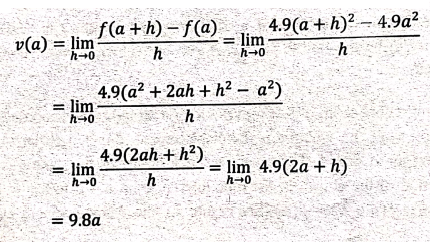
 = 9.8a

(a) The velocity after 5 s is v(5) = (9.8) (5) = 49m/s.

(b) Since the observation deck is 450 m above the ground, the ball will hit the ground at the time t₁ when s(t₁) = 450, that is,

4.9 t₁²=450

t₁²=450/4.9

t₁=√[450/4.9]

≈ 9.6s

The velocity of the ball as it hits the ground is therefore

450

v(t₁) = 9.8t₁ = 9.8 √[450/4.9] ≈ 94 m/s

 

Example 125. The position of a particle is given by the equation

s = f(t) = t³ ‒ 6t² + 9t

where t is measured in seconds and s in meters

(a) Find the velocity at time t.

(b) What is the velocity after 2 s? After 4 s?

(c) When is the particle at rest?

(d) When is the particle moving forward (that is, in the positive direction)?

(e) Draw a diagram to represent the motion of the particle.

(f) Find the total distance traveled by the particle during the first five seconds.

(g) Find the acceleration at time t and after 4 s.

(h) Graph the position, velocity, and acceleration functions for 0 ≤t≤5.

(i) When is the particle speeding up? When is it slowing down?

Solution:

(a) The velocity function is the derivative of the position function

 s = f(t) = t³ − 6t² + 9t

 v(t) = ds/dt = 3t²‒12t+9

(b) The velocity after 2 s means the instantaneous velocity when t = 2,

that is,

v(2) = (ds/dt)|_t=2= 3(2)²‒12(2)+9 = ‒3 m/s

The velocity after 4 s is

v(4) = 3(4)² – 12(4)+9 = 9 m/s

(c) The particle is at rest when v(t) = 0, that is,

3t²‒12t+9= 3(t²‒4t+3)= 3(t − 1)(t − 3) = 0

and this is true when t = 1 or t = 3. Thus the particle is at rest after 1 s and after 3

s.

(d) The particle moving in the positive direction when v(t) > 0, that is

3t²‒12t+9 = 3(t − 1)(t −3) > 0

This inequality is true when both factors are positive (t > 3) or when both factors are negative (t < 1). Thus the particle moves in the positive direction in the time intervals t < 1 and t > 3. It moves backward (in the negative direction) when 1<

t< 3.

(e) Using the information from part (d) we make a schematic sketch in the following figure of the motion of the particle back and forth along a line (the s‒ axis).

(f) Because of what we learned in parts (d) and (e), we need to calculate the distances traveled during the time intervals [0, 1], [1, 3], and [3, 5] separately. The distance traveled in the first second is

|f(1)‒f(0)| = |4‒0| = 4m

From t = 1 to t = 3 the distance traveled is

|f(3)‒f(1)| = |0‒4| = 4m

From t = 3 to t = 5 the distance traveled is

|f(5) ‒ƒ(3)| = |20‒1| = 20m

The total distance is 4 + 4 +20= 28m.

(g) The acceleration is the derivative of the velocity function:

 a(t) = d²s/dt² = dv/dt = 6t‒12

 a(4)=6(4) ‒ 12 = 12m/s²

(h) The following figure shows the graphs of s, v, and a.

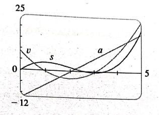
(i) The particle speeds up when the velocity is positive and increasing (v and a are both positive) and also when the velocity is negative and decreasing (v and a are both negative). In other words, the particle speeds up when the velocity and acceleration have the same sign. (The particle is pushed in the sake direction it is moving). From the above figure we see that this happens when 1 < t < 2 and when t> 3. The particle slows down when v and a have opposite signs, that is, when 0≤t<1 and when 2<t<3. The following figure summarizes the motion of the particle.