Limit of a function

LIMIT OF A FUNCTION

 

The limit of a function describes the behavior of the function when the variable is near, but does not equal, a specified number. If the values of f(x) get closer, as close as we want, to one number L as we take values of x very close to (but not equal to) a number a, then we say that "the limit of f(x), as x approaches a, equals L" and we write

  lim_x→a f(x) = L.

An alternative notation for lim_x→af(x) = L is f(x) → L as x → a which is usually read "f(x) approaches L as x approaches a".

 

 

1. ONE SIDED LIMITS

 

Consider the Heaviside unit step function H defined by H(t) = 

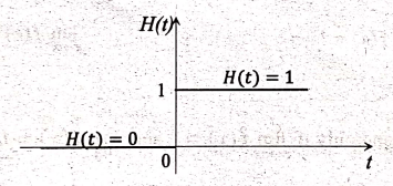
From the definition of the function and from the graph, H(t) approaches 0 from the left and H(t) approaches 1 as t approaches 0 from the right.

The limits can be written as

lim _t→0‒ H(t) and lim _t→o+ H(t).

The symbol "t→0^‒" represents that the only values of t that are less than 0 have to be considered. Similarly "t → 0+" represents that the only values of t that are greater than 0. The limit that is considered when the values of t are only less than 0 is known as the left limit and the limit that is considered when the values of t are greater than or equal to 0 is known as right limit.

In general, the left and right limits are defined as follows.

 

Definition:

The left limit as x approaches as of f(x) is L if the values of f(x) gets as close to L as when x is very close to left of a,

For x <a, lim _x→a‒ f(x) = L.

The right limit, written with a+, requires that x lies on the right of a,

For x > a, lim _x→a+ f(x) = L

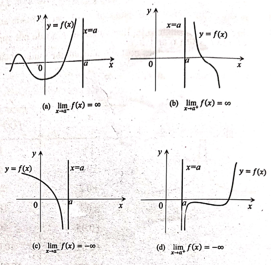
Note: Remembering that x→a^‒ means that the only values of x that are less than a are considered, and similarly x→a⁺ at means that only values satisfying x>a. Illustrations of these cases are given in the following figure

Theorem:

lim_x→α f(x) = L if and only if lim _x→α‒ f(x) = L and lim _x→α+ f(x) = L

 

 

2. INFINITE LIMITS

 

Definition: Let f be a function defined on both sides of "a", except possibly at

"a" itself. Then lim _x→a f(x) = ∞ means that the values of f(x) can he made arbitrarily large (as large as we please) by taking x sufficiently close to a, but not equal to a.

Another notation for lim _x→α f(x) = ∞ is f(x) → ∞ as x → a.

Again, the symbol ∞ is not a number, but the expression lim _x→α ƒ(x) = ∞ is often read as

"the limit of f(x), as x approaches a, is infinity"

or "f(x) becomes infinite as x approaches a"

or "f(x) increases without bound as x approaches a"

Consider the function f(x)=1/x². As x becomes close to 0, x² also becomes close to 0, and f(x) becomes very large and the same may be observed from the following table. In fact, it appears from the graph of the function f(x) = 1 / x² shown in the following figure, that the values of f(x) can be made arbitrarily large by taking x close enough to 0. Thus the values of f(x) do not approach a number, so lim _x→0 f(x) = lim _x→0 1/x² does not exist. To indicate the kind of behavior, it is written using the notation lim _x→0ƒ(x) = 1/x² =  ∞.

 

Definition: Let f be a function defined on both sides of a, except possibly at a itself. Then lim _x→a f(x) = ‒∞ means that the values of f(x) can be made arbitrarily negative large by taking x sufficiently close to a, but not equal to a.

The symbol lim _x→a f(x) = ‒∞ can be read as "the limit of f(x), as x approaches a, is negative infinity" or "f(x) decreases without bound as x approaches a".

Now consider the function f(x) = ‒ 1/x². As x→0, f(x)→ ‒∞.

Symbolically, it writes as lim _x→0 (‒1/x²) = x².

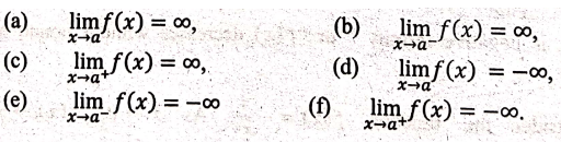
Similar definitions can be given for the one‒sided infinite limits.

lim _x→a^‒ f(x) = ∞, lim _x→a+ f(x) = ∞, lim _x→a^‒ f(x) = −∞, lim _x→a⁺ f(x) = −∞

Illustrations of these cases are given in the following figure

Note:

If lim _x→a f(x) = ∞ or lim _x→a f(x) = ‒∞, then we say lim _x→a f(x) does not exists.

 

Definition:

The vertical line x = a is called a vertical asymptote of the curve y = f(x) if at least one of the following statements is true:

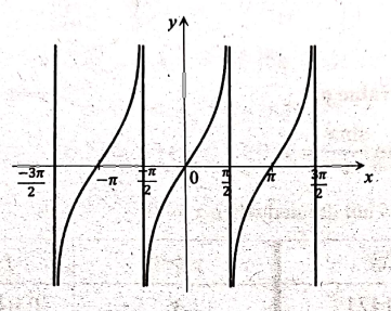
Consider the function f(x) = tan x. Because tanx = sinx / cosx, the vertical asymptotes are defined by cos x = 0, cos x → 0 as x→(π/2)⁺, whereas sin x is positive when x is near π/2, Therefore,

This shows that the line x = π/2 is a vertical asymptote. Similar reasoning shows that the lines x = ±(2n+1) π/2, where n is an integer, are all vertical asymptotes of f(x) = tanx and it can be confirmed from the graph of the function presented in the following figure.

 

Example 36. Evaluate lim_x→1(x²‒1) / (x‒1) without simplifying it.

Solution:

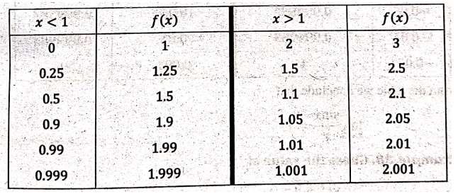
From the table we conclude that

 

Example 37. Guess the value of

lim_x→0 Sinx/x = 1

The function f(x) = sin x / x is not defined when x = 0.

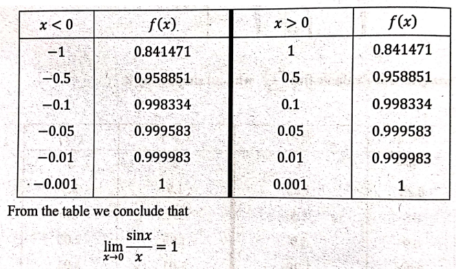
lim_x→0 Sinx/x = 1

 

Example 38. Guess the value of

 

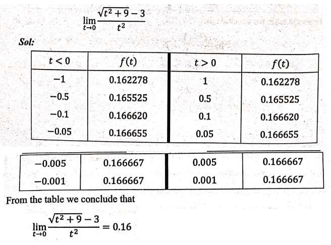
Example 39. Guess the value of the limit (if it exits) for the function lim_x→0 [ e^5x‒1 / x ] = 5 by evaluating the function at the given number x = ±0.5, ±0.1, ±0.01, ±0.001, ±0.0001 (correct to six decimal places)

Solution: The function f(x) = lim _x→0 [ e^5x‒1 / x ] is not defined when x = 0.

From the table we conclude that

lim_x→0 [ e^5x‒1 / x ] = 5

 

Example 40. Investigate

lim _x→0 sin (π/x)

Solution: The function sin x is bounded and |sin x| ≤ 1. Therefore, the given function sin (π/x) is also bounded maximum and minimum values of sin (π/x) is ±1. This can be attained by the function, if

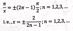
As n becomes large the value x is closer to 0 and in the neighborhood of x= 0, the value of the function sin (π/x) is either ‒1 or +1. That is, the values of the function near 0 oscillates between ‒1 and +1.

The property of function is presented graphically in Fig. and the oscillation of the function between ‒1 and +1. Hence, the limit does not exist.

 

Example 41. Sketch the graph of the function f(x) = 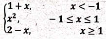 and use it to determine the values of "a" for which lim _x→a f(x) exists.

Solution: From the graph, it is observed that lim _x→a f(x) exists for all "a" except when a = −1, since the right and left limits are different at a = ‒1.

 

Example 42.

Sketch the graph of the function f(x) = 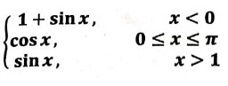 and use it to determine the values of "a" for which lim _x→a ƒ(x) exists.

Solution: From the graph, it is noticed that lim _x→a f(x) exists for all "a" except when a = π, since the left and right limits are different at the point a = π.

 

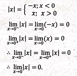
Example 43. Show that lim _x→0 |x| = 0

Solution:

 

Example 44. Prove lim _x→a |x|/x does not exist.

Solution:

 

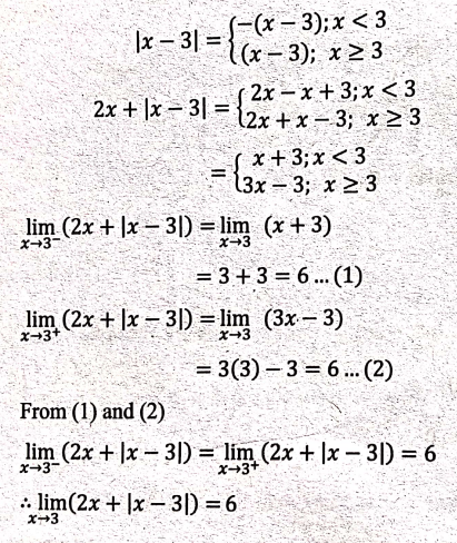
Example 45. Find the limit lim_x→3(2x+|x‒3|) if it exits. If the limit does not exist. Explain why?

Solution:

 

Example 46. Find the limit lim _x→3( 3x+9 / |x+3| ) if exits. If the limit does not exits. explain why?

Solution:

 

Definition: [[x]] is defined by the largest integer is less than or equal to [[x]] is called as greatest integer function.

eg: [[4]] = 4

[[4.3]] = 4

[[−1.5]] = −2

 

Example 49. Draw the graph of f(x) = [[x]] and show that lim _x→3[[x]] does not exists.

0 ≤x≤1⇒ [[x]] = 0

1 < x < 2 ⇒ [[x]] =1

‒1≤x<0= [[x]] = ‒1

 

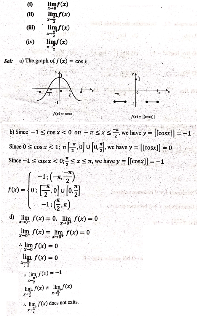
Example 50. Draw the graph of f(x) = [[cosx]] ‒ π ≤ x ≤π.

a) Sketch the graph of ƒ (x)

b) Evaluate each limit, if it exists.

c) For what values of a does lim _x→af(x) exist.

 

Example 51. Determine the infinite limit.

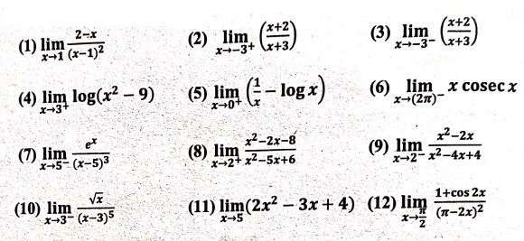
Solution:

(1) lim_x→1 [2‒x] / (x−1)² =  1/0 = ∞

(2) lim _x→3⁺( x+2 / x+3 )

Given x→‒3⁺. x is close to ‒3 but larger than ‒3.

Let x = ‒2.9

The Numerator x + 2 becomes negative.

The Denominator x + 3 becomes positive.

lim _x→3⁺( x+2 / x+3 ) = ‒∞

(3) lim _x→3^‒( x+2 / x+3 )

Given x→3^‒. x is close to ‒3 but smaller than ‒3.

Let x = ‒3.1

The Numerator x + 2 becomes negative.

The Denominator x + 3 becomes negative.

lim _x→3^‒( x+2 / x+3 ) = ∞

(4) lim_x→3⁺ log(x² ‒ 9)

Given x→ 3⁺. x is close to 3 but larger than 3.

Let x = 3.1

log(x² ‒ 9) becomes negative.

lim_x→3⁺ log(x² ‒ 9) = −∞

(5) lim_{x → 0}⁺ ( 1/x ‒ logx ) = lim _{x → 0}⁺ ( [1‒xlogx] / x )

Given x → 0⁺. x is close to 0 but larger than 0.

Let x = 0.1

The Numerator (1‒ x logx) becomes positive.

The Denominator x becomes positive.

lim _x→0⁺ (1/x ‒ logx) =∞

(6) 

Given x → (2π) ̄. x is close to 2π but smaller than 2л.

x lies in the fourth quardrant.

The Denominator sin x becomes negative.

The Numerator x becomes positive.

lim_x→(2π)^‒ x cosecx = ‒∞

(7) 

Given x→ 5^‒. x is close to 5 but smaller than 5.

Let x = 4.9

The Numerator e^x becomes positive.

The Denominator (x‒5)³ becomes negative.

 = ‒∞

(8) 

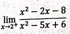
Given x → 2⁺. x is close to 2 but larger than 2.

Let x = 2.1

The Numerator x² ‒ 2x ‒ 8 becomes negative.

The Denominator x²‒5x+6 becomes negative.

 = ∞

(9) 

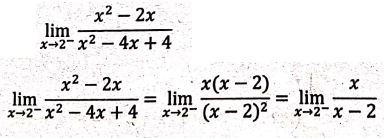
Given x → 2^‒. x is close to 2 but smaller than 2.

Let x 1.9

The Numerator x becomes positive.

The Denominator x‒2 becomes negative.

 = ‒∞

 (10) 

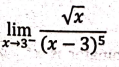
Given x→3^‒. x is close to 3 but smaller than 3.

Let x = 2.9

The Numerator √x becomes positive.

The Denominator (x‒3)⁵ becomes negative.

= ‒∞

(11) lim_x→5(2x² ‒ 3x + 4)

lim_x→5(2x² ‒ 3x + 4) = 2(5)² ‒ 3(5) + 4

=2(25) ‒ 15+4

= 50 ‒ 15+ 4 = 54 ‒ 15 = 39

 (12) 

 

Example 52. Evaluate lim_x→∞ [3x²‒x‒2] / [5x²+4x+1]

Solution: As x becomes large, both numerator and denominator become large, so it isn't obvious what happens to their ratio. We need to do some preliminary algebra.

To evaluate the limit at infinity of any rational function, we first divide both the numerator and denominator by the highest power of x that occurs in the denominator. (We may assume that x ≠ 0, since we are interested only in large values of x.) In this case the highest power of x in the denominator is x², so we have

 

Example 53. Find lim_x→∞[x²+x] / [3‒x]

Solution:

We divide the numerator and denominator by the highest power of x in the denominator, which is just x:

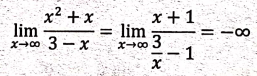
because x + 1→ ∞ and 3/x ‒1→ ‒1 as x → ∞

 

 

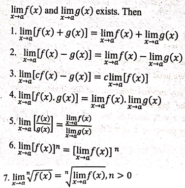
3. CALCULATING LIMIT USING LIMIT LAWS.

 

Suppose that c is a constant and the limit

 

Example 54. Given that lim_x→2f(x) = 4; lim_x→2g(x) = ‒2 find the limit that exists from the following. If the limits does not exists explain why.

 

EXERCISE

 

4. ASYMPTOTES

 

Unlike polynomials whose graphs are continuous (unbroken) curves, the graphs of rational functions have discontinuities at the points where the denominator is zero. Unlike polynomials, rational functions may have numbers at which they are not defined. Near such points, many rational functions have graphs that closely

approximate a vertical line, called a vertical asymptote.

 

HORIZONTAL ASYMPTOTE

Unlike the graphs of non‒constant polynomials, which eventually rise or fall indefinitely, the graphs of many rational functions eventually get closer and closer to some horizontal line, called a horizontal asymptote.

 

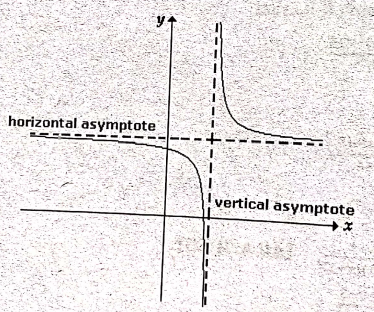
Example 74. Find the horizontal and vertical asymptotes of the graph of the function

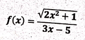
Solution: Dividing both numerator and denominator by x and using the properties of limits, we have

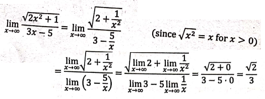
Therefore the line y = √2/3 is a horizontal asymptote of the graph of f.

In computing the limit as x → ‒∞, we must remember that for x < 0, we have √x² = |x| = ‒x. So when we divide the numerator by x, for x < 0 we get

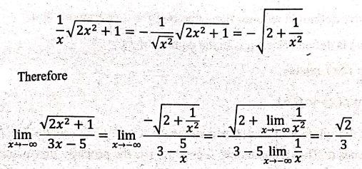
Thus the line y = −√2/3 is also a horizontal asymptote.

A vertical asymptote is likely to occur when the denominator, 3x‒5, is 0, that is, when x = 5/3. If x is close to 5/3 and x > 5/3, then the denominator is close to 0 and 3x‒5 is positive. The numerator √[2x²+1] is always positive, so f(x) is positive. Therefore

If x is close to 5/3 but x < 5/3, then 3x‒5< 0 and so f(x) is large negative. Thus

The vertical asymptote is x = 5/3. All three asymptotes are shown in Figure 8.