Karnaugh Map Minimization

Karnaugh Map Minimization

In the previous section we have seen that for simplification of Boolean expressions by Boolean algebra we need better understanding of Boolean laws, rules and theorems. During the process of simplification we have to predict each successive step. For these reasons, we can never be absolutely certain that an expression simplified by Boolean algebra alone is the simplest possible expression. On the other hand, the map method gives us a systematic approach for simplifying a Boolean expression. The map method, first proposed by Veitch and modified by Karnaugh, hence it is known as the Veitch diagram or the Karnaugh map.

1. One–Variable, Two–Variable, Three–Variable and Four–Variable Maps

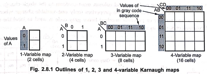
The basis of this method is a graphical chart known as Karnaugh map (K–map). It contains boxes called cells. Each of the cell represents one of the 2ⁿ possible products that can be formed from n variables. Thus, a 2–variable map contains 2² = 4 cells, a 3–variable map contains 2³ = 8 cells and so forth. Fig. 2.8.1 shows outlines of 1, 2, 3 and 4–variable maps.

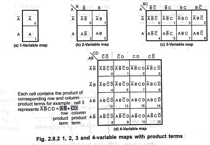
Product terms are assigned to the cells of a Karnaugh map by labeling each row and each column of the map with a variable, with its complement, or with a combination of variables and complements. The product term corresponding to a given cell is then the product of all variable in the row and column where the cell is located. Fig. 2.8.2 shows the way to label the rows and columns of a 1, 2, 3 and 4–variable maps and the product terms corresponding to each cell.

It is important to note that when we move from one cell to the next along any row or from one cell to the next along any column, one and only one variable in the product term changes (to a complemented or to an uncomplemented form). For example, in Fig. 2.8.2 (b) the only change that occurs in moving along the bottom row from A to AB is the change from  to B. Similarly, the only change that occurs in moving down the right column from ĀB to AB is the change from Ā to A, Irrespective of number of  variables the labels along each row and column must conform to the single–change rule. We know that the gray code has same properties (only one variable change when we proceed to next number or previous number) hence gray code is used to label the rows and columns of K–map as shown in Fig. 2.8.3.

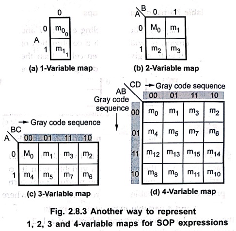
Fig. 2.8.3 shows label of the rows and columns of a 1, 2, 3 and 4–variable maps using gray code and the product terms corresponding to each cell. Here, instead of writing actual product terms, corresponding shorthand minterm notations are written in the cell and row and columns are marked with gray code instead of variables.

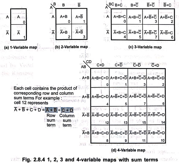
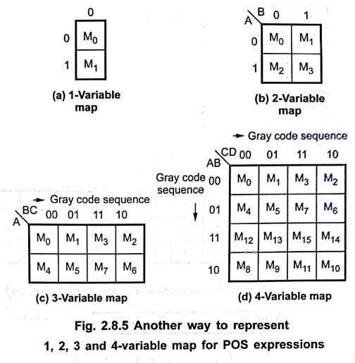
In case of POS expressions we assign maxterms (sum terms) to the cells of a Karnaugh map. Fig. 2.8.4 shows the way to label the rows and columns of a 1, 2, 3 and 4–variable maps and the sum terms corresponding to each cell. Fig. 2.8.4 shows label of the rows and columns of 1, 2, 3 and 4–variable maps using gray code and the sum terms corresponding to each cell. Here, instead of writing actual sum terms, corresponding shorthand maxterm notations are written in the cell and row and columns are marked with gray code instead of variables.

2. Plotting a Karnaugh Map

We know that logic function can be represented in various forms such as truth table, SOP Boolean expression and POS Boolean expression. In this section we will see the procedures to plot the given logic function in any form on the Karnaugh map.

1. Representation of Truth Table on Karnaugh Map

Cell : The smallest unit of a Karnaugh map, corresponding to one line of a truth table. The input variables are the cell's co–ordinates and the output variable is the cell's contents.

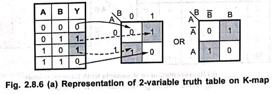
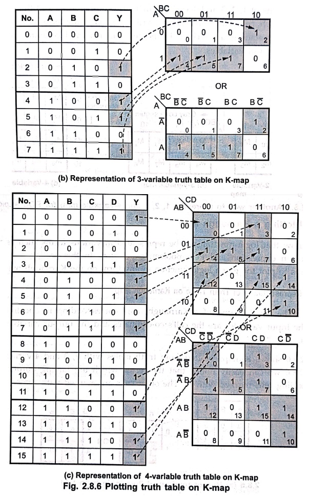
Fig. 2.8.6 shows K–maps plotted from truth tables with 2, 3 and 4–variables. Looking at Fig. 2.8.6 we can easily notice that the terms which are having output 1, have the corresponding cells marked with 1s. The other cells are marked with zeros.

Note : The student can verify the data in each cell by checking the data in the column Y for particular row number and the data in the same cell number in the K–map.

2. Representing Standard SOP on K–Map

A Boolean expression in the sum of products form can be plotted on the Karnaugh map by placing a 1 in each cell corresponding to a term (minterm) in the sum of products expression. Remaining cells are filled with zeros. This is illustrated in the following examples.

Examples for Understanding

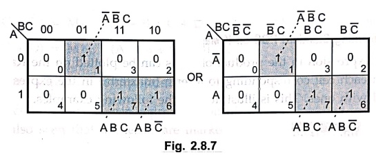
Example: 1

Plot Boolean expression  on the Karnaugh map.

Solution :

The expression has 3–variables and hence it can be plotted using 3–variable as in Fig. 2.8.7.

Example: 2

Simplify the following expression using K–map method.

Y = Σm(7, 9, 10, 11, 12, 13, 14, 15)

Solution :

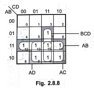
Y = AB + AC + AD + BCD

Example: 3

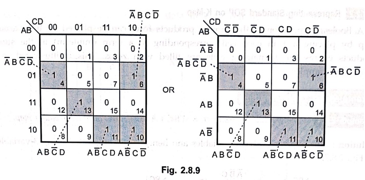
Plot Boolean expression

 on the Karnaugh map.

Solution :

The expression has 4–variables and hence it can be plotted using 4–variable map as shown in Fig. 2.8.9.

3. Representing Standard POS on K–Map

A Boolean expression in the product of sums can be plotted on the Karnaugh map by placing a 0 in each cell corresponding to a term (maxterm) in the expression. Remaining cells are filled with ones. This is illustrated in the following examples.

Examples for Understanding

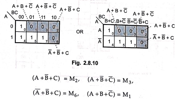
Example: 4

Plot Boolean expression  on the Karnaugh map.

Solution :

The expression has 3–variables and hence it can be plotted using 3–variable map as shown in Fig. 2.8.10.

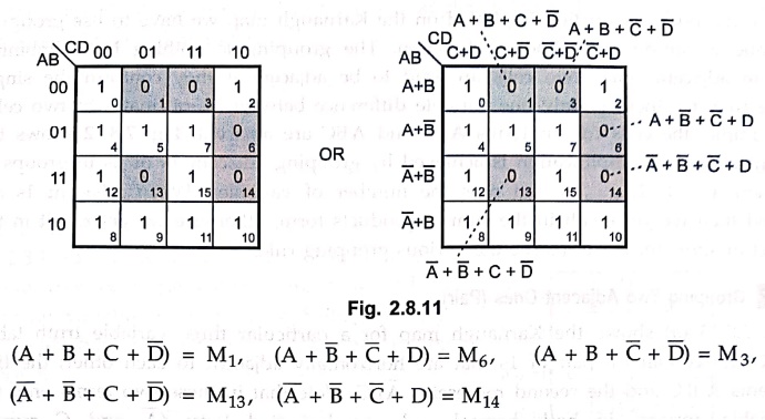
Example: 5

Plot Boolean expression.

Solution :

The expression has 4–variables and hence it can be plotted using 4–variable map as shown in Fig. 2.8.11.

3. Grouping Cells for Simplification

In the last section we have seen representation of Boolean function on the Karnaugh map. We have also seen that minterms are marked by 1s and maxterms are marked by 0s.

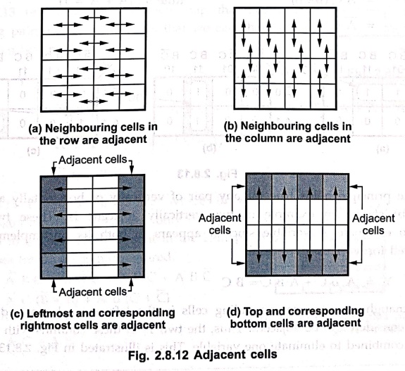
Once the Boolean function is plotted on the Karnaugh map we have to use grouping technique to simplify the Boolean function. The grouping is nothing but combining terms in adjacent cells. Two cells are said to be adjacent if they conform the single change rule. i.e. there is only one variable difference between co–ordinates of two cells. For example, the cells for minterms ABC and ĀBC are adjacent. Fig. 2.8.12 shows the adjacent cells. The simplification is achieved by grouping adjacent 1s or 0s in groups of 2ⁱ, where i = 1, 2, n and n is the number of variables. When adjacent 1s are grouped then we get result in the sum of products form; otherwise we get result in the product of sums form. Let us see the various grouping rules.

1. Grouping Two Adjacent Ones (Pair)

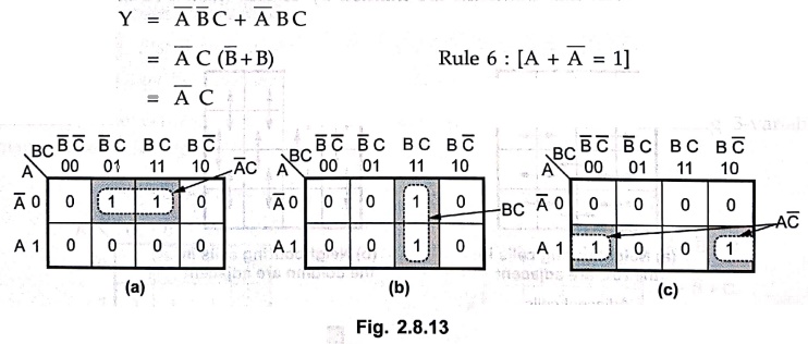
Fig. 2.8.13 (a) shows the Karnaugh map for a particular three variable truth table. This K–map contains a pair of 1s that are horizontally adjacent to each other; the first represents C and the second represents BC. Note that in these two terms only the B variable appears in both normal and complemented form ( and C remain unchanged). Thus these two terms can be combined to give a resultant that eliminates the B variable since it appears in both uncomplemented and complemented form. This is easily proved as follows :

This same principle holds true for any pair of vertically or horizontally adjacent 1s. Fig. 2.8.13 (b) shows an example of two vertically adjacent 1s. These two can be combined to eliminate A variable since it appears in both its uncomplemented and complemented forms. This gives result

Y =  B C + A B C = B C

In a Karnaugh map the corresponding cells in the leftmost column and rightmost column are considered to be adjacent. Thus, the two 1s in these columns with a common row can be combined to eliminate one variable. This is illustrated in Fig. 2.8.13 (c).

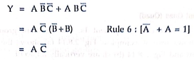
Here variable B has appeared in both its complemented and uncomplemented forms and hence eliminated as follows:

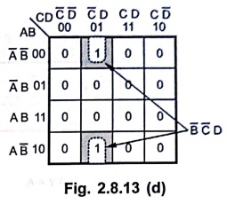
Let us see another example shown in Fig. 2.8.13 (d). Here two 1s from top row and bottom row of some column are combined to eliminate variable A, since in a K–map the top row and bottom row are considered to be adjacent.

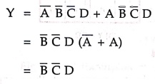
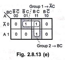
Fig. 2.8.13 (e) shows a Karnaugh map that has two overlapping pairs of 1s. This shows that we can share one term between two pairs.

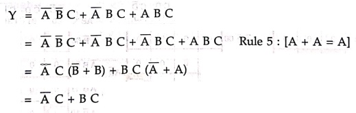
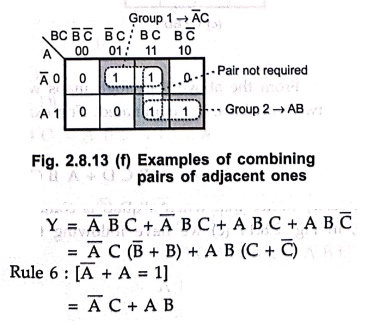
Fig. 2.8.13 (f) shows a K–map where three group of pairs can be formed. But only two pairs are enough to include all 1s present in the K–map. In such cases third pair is not required.

A pair is a group of two adjacent cells in a Karnaugh map. It cancels one variable in a K–map simplification.

2. Grouping Four Adjacent Ones (Quad)

In a Karnaugh map we can group four adjacent 1s. The resultant group is called Quad. Fig. 2.8.14 shows several examples of quads. Fig. 2.8.14 (a) shows the four 1s are horizontally adjacent and Fig. 2.8.14 (b) shows they are vertically adjacent.

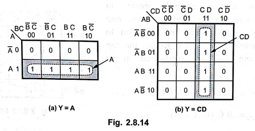
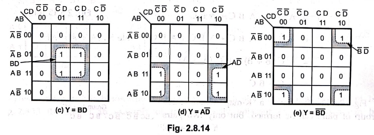
A K–map in Fig. 2.8.14 (c) contains four 1s in a square and they are considered adjacent to each other. The four 1s in Fig. 2.8.14 (d) are also adjacent, as are those in Fig. 2.8.14 (e) because, as mentioned earlier, the top and bottom rows are considered to be adjacent to each other and the leftmost and rightmost columns are also adjacent to each other.

From the above Karnaugh maps we can easily notice that when a quad is combined two variables are eliminated. For example, in Fig. 2.8.14 (c) we have following terms with 4 variables :

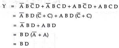
(Only two variables in the result, variables A and C are eliminated)

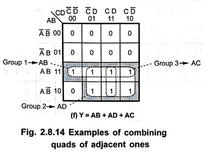
Fig. 2.8.14 (f) shows overlapping groups. As mention earlier one term can be shared between two or more groups.

Quad is a group of four adjacent cells in a Karnaugh map. It cancels two variables in a K–map simplification.

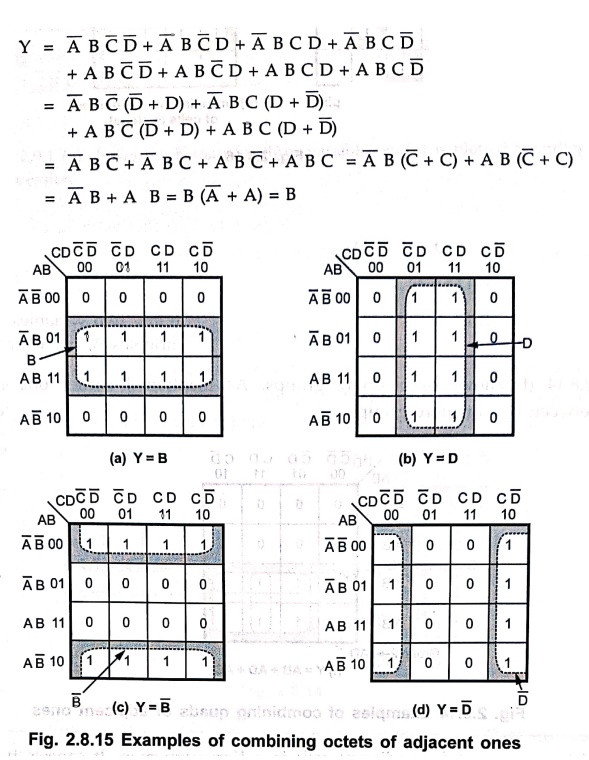
3. Grouping Eight Adjacent Ones (Octet)

In a Karnaugh map we can group eight adjacent 1s. The resultant group is called as octet. Fig. 2.8.15 shows several examples of octets. Fig. 2.8.15 (a) shows the eight 1s are horizontally adjacent and Fig. 2.8.15 (b) shows they are vertically adjacent.

From Fig. 2.8.15 we easily observe that when an octet is combined in a four variable map, three of the four variables are eliminated because only one variable remains unchanged. For example, in K–map shown in Fig. 2.8.15 (a) we have following terms :

Octet is a group of eight adjacent cells in a Karnaugh map. It cancels three variables in a K–map simplifications.

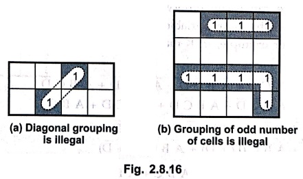
4. Illegal Grouping

Fig. 2.8.16 shows the examples of illegal grouping of cells.