Applied Calculus: UNIT III: Integral Calculus
The area problem
Integral Calculus
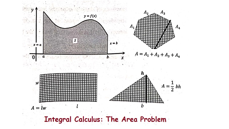
Explanation, Formula, Equation, Example and Solved Problems - Integral Calculus: The area problem
THE
AREA PROBLEM
Let as first attempt to
solve the area problems given a function f
that is continuous and non‒negative on an intervals [a, b] find the area
between the graph of f and the
intervals [a, b] on the x-axis.
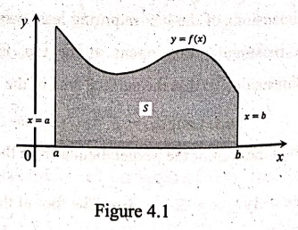
This means that S,
illustrated in is bounded by the graph of a continuous function f[where f(x) ≥ 0], the vertical lines x = a and x = b and the x-axis
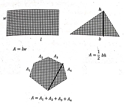
For a rectangle, the
area is defined as the product of the length and the width. The area of the
triangle is half the base times the height.
The area of the polygon
is found by dividing it into triangles adding the areas of the triangles.
However it is not so
easy to find the area of a region with curved sides. But part of the area
problem is to make this intuitive idea precise by giving an exact definition of
area.
Recall that defining a
tangent we first approximated the slope of the tangent line by slope of secant
lines and then we took the limit of these approximations
We pursue a similar
idea for areas. We first approximate the regions S by the rectangular and then
we take the limit of the areas of these rectangular as we increases the number
of rectangular.
The concept conceived
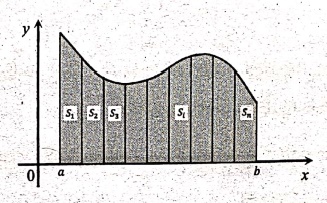
from the above example may be applied to the more general region S shown in the
figure 4.1 subdividing the region S into n
scripts S1, S2, ..., Sn of equal width as in
figure 4. 2.
The width of the
interval [a, b] is b ‒ a, so the width of the each of the n scripts
∆x =
(b‒a) / n
These scripts divide
the intervals [a, b] into n sub
intervals.
[x0, x1], [x1,
x2], [x2, x3], ..., [xn‒1,xn],
where x0 = a and xn=b
The right endpoints of
the subintervals are x1 = a + ∆x, x2 = a + 2∆x + ...,xn
= a + n∆x let's approximate the ith
strip Si by a rectangle with width ∆x and height f(xi) which is the value of f at the right endpoints.
Then the area of the ith rectangle is f(xi)∆x. Therefore, the area
S is approximated by the sum of the area of these rectangles and is given by
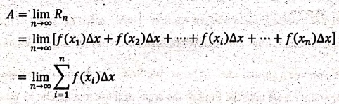
Rn = f(x1)∆x + f(x2)∆x + ….. + f(xi)∆x + ….. + f(xn)∆x
As n→ ∞, Rn→
A (Area of S)
Definition
The area A of the
region S that lies under the graph of the continuous function f is the limit of the sum of the areas
of approximation rectangles:
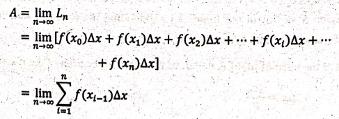
Similarly, assuming
that f is continuous, the area A of S
can be obtained by considering the rectangles with left endpoints as given
below
Instead of using left
endpoints or right endpoints, we could take the height of the ith rectangle
to be the value of f at any number xi* in the ith subinterval
[xi‒1,x¡].
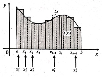
We call the number x1*,
x*2, ..., xn*
the sample points as shown in figure 4.3. So more general expressions for the
area of the S is
A = limn→∞ [ f(x1*)∆x + f(x2*)∆x + ….. + f(xi*)∆x + …. + f(xn*)∆x ]
Example
1. Find the approximate area L4 and R4 for f(x) = x2 between x = 0 and x = 1.
Solution:
Given that f(x) = x2, a = 0, b = 1 and n = 4.
∆x = (b‒a)/n = (1‒0) /
4 = 1/4
Hence the interval is
subdivided into four equal parts as
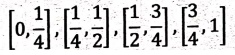
The left end points are
0,1/4,1/2,3/4.
The right end points
are 1/4,1/2,3/4,1
The values of the
function at left end points of the intervals are
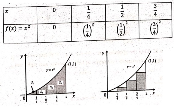
The sum of the areas of
the lower approximate rectangles is
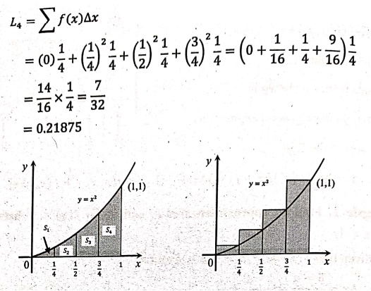
The values of the
function at right end points of the intervals are
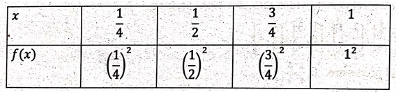
The sum of the areas of
the upper approximate rectangles is
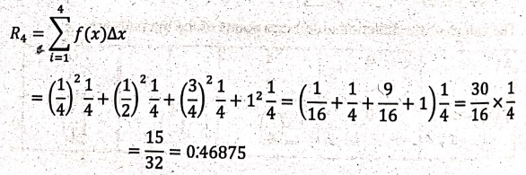
= 15/32 = 0.46875
Example
2. Find the approximate area for f(x)
= x2 between x = 0 and x =
1 using eight approximate rectangles at left endpoints and right end‒points.
Solution:
Given that f(x) = x2, a = 0, b = 1 and n = 8.
∆x = (b‒ a)/n = (1‒0) /
8 = 1/8
Hence the interval is
subdivided into eight parts as
[0,1/8],[1/8,2/8], …,
[7/8,1]
The left end points are
0,1/8,2/8, …,7/8
The right end points
are
1/8,2/8, …,7/8,1
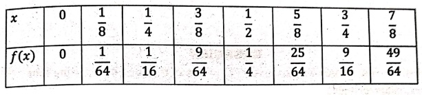
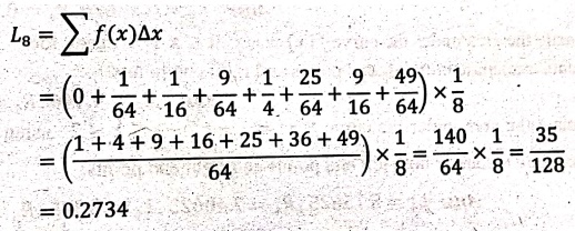
To find L8:
The values of the
function at the left end points of the intervals are
The sum of the areas of
the lower approximate rectangles is
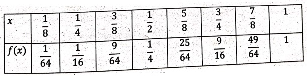
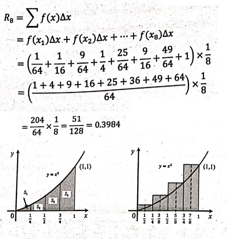
To find R8:
The values of the
function at the right end points of the intervals are
The sum of the areas of
the upper approximate rectangles is
EXERCISE
1. Estimate the area
under the curve f(x) = cos x 0 ≤ x ≤ π/2 using four approximate
rectangle both left end points and right end points.
Ans:
L4=0.3767π, R4 = 0.2516π.
2. Estimate the area
under the curve f(x) = √x 0 ≤ x ≤ 4
using four approximate rectangle both left end points and right end points.
Ans: L4 =
4.146, R4 = 6.146.
3. Estimate the area
under the curve f(x)=1+x2
‒1≤ x ≤2 using four and six approximate rectangle both left end
points and right end points.
Ans:
L4=5.15625, R4 = 7.40625, L6 = 5.375, R6
= 6.875.
4. Evaluate the upper
and lower sum for f(x) = 1 / (1+x2) 0≤x≤1 with n = 10.
Ans:
L10=0.75998, R10 = 0.80998.
Applied Calculus: UNIT III: Integral Calculus : Tag: Applied Calculus : Integral Calculus - The area problem
Applied Calculus: UNIT III: Integral Calculus
Under Subject

Applied Calculus
MA25C01 Maths 1 M1 - 1st Semester | 2025 Regulation | 1st Semester 2025 Regulation
Related Subjects

English Essentials I
EN25C01 1st Semester | 2025 Regulation | 1st Semester 2025 Regulation

தமிழர் மரபு - Heritage of Tamils
UC25H01 1st Semester | 2025 Regulation | 1st Semester 2025 Regulation
Applied Calculus
MA25C01 Maths 1 M1 - 1st Semester | 2025 Regulation | 1st Semester 2025 Regulation

Applied Physics I
PH25C01 1st Semester | 2025 Regulation | 1st Semester 2025 Regulation

Applied Chemistry I
CY25C01 1st Semester | 2025 Regulation | 1st Semester 2025 Regulation

Makerspace
ME25C04 1st Semester | 2025 Regulation | 1st Semester 2025 Regulation

Computer Programming C
CS25C01 1st Semester | 2025 Regulation | 1st Semester 2025 Regulation

Computer Programming Python
CS25C02 1st Semester | 2025 Regulation | 1st Semester 2025 Regulation

Fundamentals of Electrical and Electronics Engineering
EE25C03 1st Semester | 2025 Regulation | 1st Semester 2025 Regulation

Introduction to Mechanical Engineering
ME25C03 1st Semester | 2025 Regulation | 1st Semester 2025 Regulation

Introduction to Civil Engineering
CE25C01 1st Semester Civil Department | 2025 Regulation | 1st Semester 2025 Regulation
Essentials of Computing
CS25C03 1st Semester - AID CSE IT Department | 2025 Regulation | 1st Semester 2025 Regulation

Applied Physics I Laboratory
PH25C01 1st Semester practical Laboratory Manual | 2025 Regulation | 1st Semester Laboratory 2025 Regulation

Applied Chemistry I Laboratory
CY25C01 1st Semester practical Laboratory Manual | 2025 Regulation | 1st Semester Laboratory 2025 Regulation

Computer Programming C Laboratory
CS25C01 1st Semester practical Laboratory Manual | 2025 Regulation | 1st Semester Laboratory 2025 Regulation

Computer Programming Python Laboratory
CS25C02 1st Semester practical Laboratory Manual | 2025 Regulation | 1st Semester Laboratory 2025 Regulation
Engineering Drawing
ME25C01 EEE Mech Dept | 2025 Regulation | 2nd Semester 2025 Regulation

Basic Electronics and Electrical Engineering
EE25C04 1st Semester ECE Dept | 2025 Regulation | 2nd Semester 2025 Regulation