The definite integral

THE DEFINITE INTEGRAL

We saw that a limit of the form

arise when we compute an area. We also saw that it arises when we try to find the distance travelled by an object. It turns out that this same type of limit occurs in a wide variety of situations even when f is not necessarily a positive function. We will see that limits of the form in above also arise in finding lengths of curves, volumes of solids, centres of mass, force due to water pressure, and work, as well as other quantities. We therefore give this type of limit a special name and notation.

Definition:

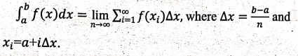
Let f be a function defined for a ≤ x ≤ b. We divide the interval [a, b] into n sub‒intervals of equal width ∆x=(b‒a)/n. Let x₀ = a, x₁, x₂, x₃ … x_n = b be the end points of these sub‒intervals. Let x₁*, x₂*, x₃*, ..., x_n* be any sample points in these sub‒intervals. So x_i* lies in the ith sub‒interval [x_i−1,x_i]. Then the definite integral of f from a to b is given by

provided that this limit exists and gives the same value for all possible points. If it exists, then f is integrable on [a, b].

Note:

• The symbol ∫ was introduced by Leibniz and is called an integral sign. It is an elongated S and was chosen because an integral is a limit of sums. In the notation, _a∫^bf(x)dx, f(x) is called the integrand and a and b are called the limits of integration, a is the lower limit and b is the upper limit. The symbol dx has no meaning by itself. _a∫^b f(x)dx is all one symbol. The dx indicates that the independent variable is x. The procedure of calculating an integral is called integration.

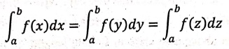
• The definite integral _a∫^b f(x)dx is a number. It does not depend on x. We can use any letter in the place of x, without changing the value of the integral.

• The sum Σ_i=1^∞f(x_i*)∆x is called a Riemann sum after the German Mathematician Bernhard Riemann. The definite integral at an integrable function can be approximated to within any desired degree of accuracy by a Riemann sum. If f is positive, then the Riemann sum can be interpreted as a sum of areas of approximating rectangles. The definite integral _a∫^b f(x)dx is interpreted as the area under the curve y = f(x) from a to b. If f takes on both positive and negative values, then the Riemann sum is the sum of the areas of the rectangles that lie above x‒axis and the negatives of the areas of the rectangles that lie below the x‒axis. A definite intégral can be interpreted as a net area, (i.e.,) a difference of areas.

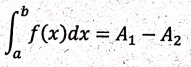
where A₁ is the area of the region above the x‒axis and below the graph of f, and A₂ is the area of the region below the x‒axis and above the graph of f.

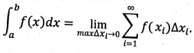
• Although we have defined _a∫^b f(x)dx by dividing [a, b] into sub‒intervals of equal width, there are situations in which it is useful to work with sub‒ intervals of unequal width. If the sub‒interval widths are ∆x₁, ∆x₂, ..., ∆x_n we have to ensure that all these widths approach 0 in the limiting process. This happens if the largest width, max ∆x_i, approaches 0. So in these case the definition of a definite integral becomes

• We have defined the definite integral for an integrable function, but not all functions are integrable.

Theorem 1:

If f is continuous on [a, b] or if f has only a finite number of discontinuities, then f is integrable on (a, b). (i.e.,) The definite integral _a∫^b f(x)dx exists.

Theorem 2:

If f is integrable on [a, b], then

Properties of definite integral:

When we defined the definite integral _a∫^b f(x)dx, we assumed that a < b. But the definition as a limit of Riemann sums makes sense even if a > b. If we reverse a and b, then ∆x changes from (b ‒ a/n) to (a – b/n)

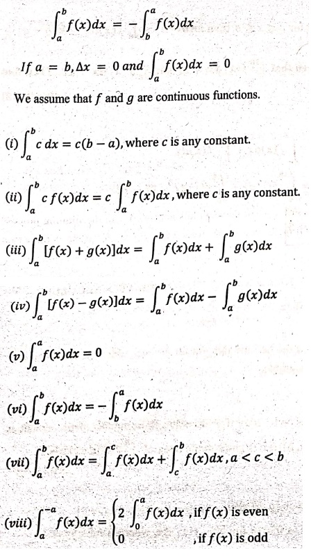
Also the comparison properties of the integral are given as follows

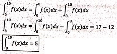
Example 3. Given that ₀∫¹⁰ f(x) dx = 17 and so ₀∫⁸ f(x) dx = 12. Then find ₈∫¹⁰ f(x) dx.

Solution: We know that

THE FUNDAMENTAL THEOREM OF CALCULUS

The Fundamental Theorem of Calculus is appropriately named because it establishes a connection between the two branches of calculus: differential calculus and integral calculus.

It gives the precise invert relationship between the derivative and the integral

ANTIDERIVATIVE

A physicist who knows the velocity of a particle might wish to know its position at a given time. An engineer who can measure the variable rate at which water is leaking from a tank wants to know the amount leaked over a certain time period. A biologist who knows the rate at which a bacteria population is increasing might want to deduce what the size of the population will be at some future time. In each case, the problem is to find a function. F whose derivative is a known function f. If such a function F exists, it is called an anti‒derivative of f.

DEFINITION:

A function F is called an antiderivative of f on an interval I if F'(x) = f(x) for all x in I.

THEOREM:

If F is an antiderivative of f on an interval I, then the most general antiderivative of f on I is

F(x) + C

where C is an arbitrary constant.

Theorem 1: The Fundamental Theorem of Integral Calculus ‒ Part 1

If f is continuous on [a, b], then the function g defined by

 g(x) = _a∫^x f(x) dx, a ≤ x ≤b

is continuous on [a, b] and differentiable on (a, b) and g'(x) = f(x).

The second part of the Fundamental Theorem of Calculus, which follows easily from the first part, provides us with a much simpler method for the evaluation of integrals.

Theorem 2: The Fundamental Theorem of Integral Calculus‒Part 2

If f is continuous on [a, b], then

_a∫^b f(x) dx = F(b) ‒ F(a)

where F is anti derivative of f, that is, a function such that F' = f

Example 4. Find the derivative of the function g(x) = _a∫^x√[1+ t²]dt.

Solution: By the fundamental theorem of calculus part I, we have

g(x) = ` _a∫^x f (t) dt,    a≤ x ≤ b

g'(x) = f(x)

The given integral is

g(x) = _a∫^x  √[t² + 1] dt

Here, f(t) = √[1 + t²] and f(x) = √[1 + x²].

Hence g'(x) = f(x) = √[1+x²].

Example 5. Find the derivative of the function using the fundamental theorem of calculus g(s) = ₅∫^S f(t ‒ t²)⁸ dt.

Solution: By the fundamental theorem of calculus part I, we have

 g(x) = _a∫^x f(t) dt,    a≤ x ≤ b

g'(x) = f(x)

The given integral is

g(s) = ₅∫^S (t − t²)⁸ dt.

Here f(t) = (t‒t²)⁸ and f(s) = (s‒s²)⁸

 g'(s) = f(s) = (s‒s²)⁸.

Example 6. Find the derivative of F(x) = _x∫^π √[1+ sect] dt

Solution:

By the fundamental theorem of calculus part 1, we have

 g(x) = _a∫^x f(t) dt, a≤ x ≤b

 g'(x) = f(x)

The given function can be rewritten as

F(x) = ‒ _π∫^x √[ 1+ sect ] dt

F'(x) = ‒√[1+ sec x]

Example 7. Find the derivative of G(x) = _x∫¹ cos √t dt.

Solution: By the fundamental theorem of calculus part I, we have

g(x)= _a∫^x f(t) dt, a≤ x ≤b

g'(x) = f(x)

The given function can be rewritten as

G(x) = ‒ ₁∫^x cos √t dt.

G'(x) = ‒ cos √x

Example 8. Find d/dx ₁∫^x4 sect dt

Solution:

By the fundamental theorem of calculus part I, we have

g(x) = _a∫^x f(t) dt, a≤x≤b

g'(x) = f(x)

The given integral is

 = sec x⁴  = sec x⁴ (4x³) = 4x³ sec x⁴.

Evaluate ₁∫³ e^x dx by fundamental theorem

Solution: The function f(x) = e^x is continuous everywhere.

By the fundamental theorem of calculus part II, F(x) = e^x,

 ₁∫³ e^x dx = F(3) − F(1) = e³ – e

Example 10. What is wrong with the calculation _‒1∫³ dx/x² = ‒ 4/3.

Solution: By property of definite integral,

_a∫^b f(x) dx ≥ 0 ⇒ f(x) ≥ 0.

Here, f(x) = 1/x² > 0 but _‒1∫³ dx/x² = ‒ 4/3 < 0

The fundamental theorem of calculus is applied to only continuous function. Here, f(x) = 1/x² is not continuous on [‒1,3]. i.c., f(x) is discontinuous at x = 0.

So, _‒1∫³ dx/x² does not exist.

Example 11. What is wrong with the calculation ₀∫^π sec² x dx = 0.

Solution:

Here f(x) = sec² x = 1 / cos²x  0≤x≤π

The fundamental theorem of calculus applied to only continuous function. Here,

 f(x)= sec² x = 1 / cos²x  is not continuous at x = π / 2, Since,

 f(π/2) = 1 / cos²(π/2) = 1/0 = ∞

At x = π/2 the function f(x) = sec²x is discontinuous.

So, ₀∫^π sec²x dx does not exist.

EXERCISE

5. What is wrong in the integral _‒2∫¹ dx/x⁴ = ‒ 3/8

Answer: The function f(x) = 1/x⁴ is not continuous at x = 0

6. What is wrong in the integral _‒1∫² 4/x³ dx = 3/2

Answer: The function f(x) = 4/x³ is not continuous at x=0

7. What is wrong in the integral _π/3∫^π secx tan x dx = ‒3

Answer: The function f(x) = secx tanx is not continuous at x = π/2