Least Square Solutions: Example Solved Problems

LEAST SQUARE SOLUTIONS

WORKED EXAMPLES

Example 1

 Find the least squares solutions of Ax=b where 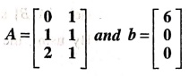 what quantity is being minimized?

Solution:

1. Compute A^TA and A^Tb

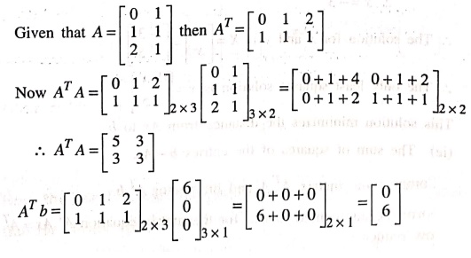
2. Form the augmented matrix

 A^TAx = A^Tb and row reduce

3. Method of solution

Now let us consider the above matrix form is in the form

 AX=B           (Here A = A^TA)

Let us apply Gauss elimination method to find the solution for x and y.

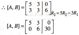
(ie) [A, B] should be converted as upper triangular matrix.

By using the back substitution method, we have

5x+3y=0

6y=30

y=30/6

y= 5

Hence

5x=−3y

x=−3/5

5x=−15

 x=−3

 The solution for x and y is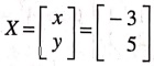 

 The only least squares solution is x = 

This solution minimizes the distance from Ax to b.

(ie) The sum of squares of the entries b−Ax.

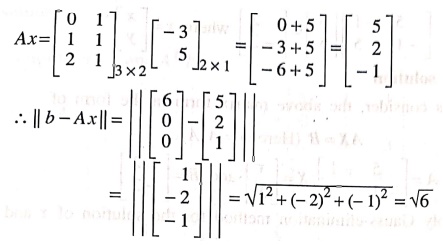
 The minimizing quantity is √6.

 

Example 2

Find the least squares solutions of Ax = b where .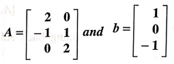

Solution:

1. Compute A^TA and A^Tb

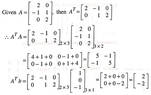
2. Form the augmented matrix

 A^TAx = A^Tb

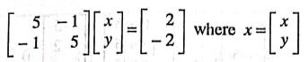
3. Method of solution

Now let us consider, the above matrix form in the form of

 AX= B               (Here A=A^TA)

where

Let us apply Gauss−elimination method for the solution of x and y.

(Convert into an upper triangular matrix)

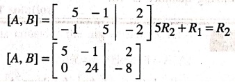
Using back substitution method, we have

5x−y=2 and 0x + 24y = −8

  24y=−8

y= − 8/24 = − 1/3

Hence 5x−y=2  ⇒ 5x=2+y   

⇒ 5x=2−(1/3)

 5x = 5/3

 x = 1/3

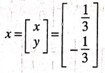
 Hence the only least squares solution is

 

Example 3

Find the least squares solutions of Ax = b where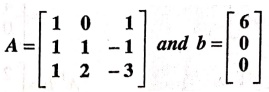 

Solution:

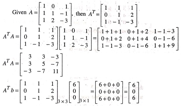
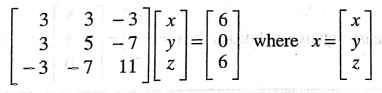
1. Compute A^TA and A^Tb

2. Form the augmented matrix

  A^TAx = A^Tb.

3. Method of solution

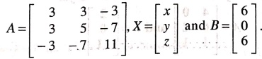
Let AX=B                (Here A = A^TA).

Let us apply Gauss−elimination method to find the solution.

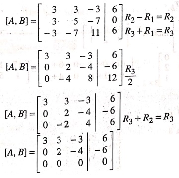
By using back substitation method, we have

3x+3y−3z=6

2y−4z=−6

0z=0

(i.e.,) x+y−z=2

y−2z=−3

Put z=0; then y=−3+2z=−3

Put z=0 and y=−3 in the first equation, we get

x=2−y+z=2+3+0

 x=5

Hence

x=5,y=−3 and z = 0

 The least squares solutions is x =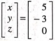 

 

Example 4

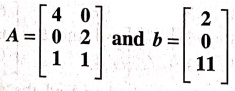
Find a least squares solutions of Ax=b for

Solution:

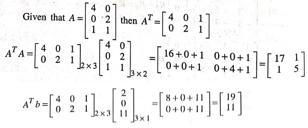
1. Compute A^TA and A^Tb.

2. Form the augmented matrix.

 A^TAx = A^Tb

3. Method of solution

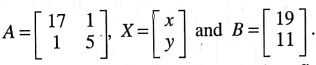
Let AX=B              (Here A = A^TA).

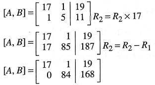
Let us apply Gauss elimination method to find the solution.

By using back substitution method we have

17x+y=19

84y = 168

y=168/84 = 2

Substitute y = 2 in, 17x+y=19 becomes

17x=19−y

⇒ x=1

  The least squares solution is x= 

 

Example 5

Find the least squares solution to

x + 2y + z = 1

3x−y=2

2x+y−z=2

x + 2y +2z=1

Solution:

This system takes the matrix form Ax=b, where

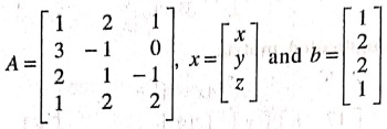
1. Compute A^TA and A^Tb

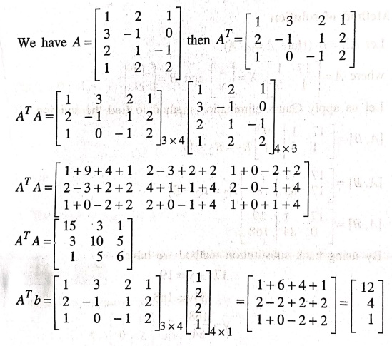
2. Form the augmented matrix

 A^TAx = A^Tb

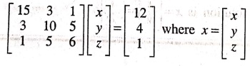
3. Method to solution

Let AX = B                (Here A= A^TA)

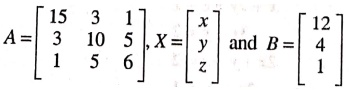
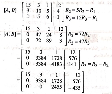
Let us apply Gauss elimination method to find the solution

By using back substitution method, we have

 15x+3y+z = 12

 384y+1728z = 576

 2455z = −435

From the last equation z = − 435/2455 = −0.177189.

Substitute z = −0.177189 in the second equation

 3384y = 576−1728z

y = 1/3384 [576−1728z]

y= 882.182592 / 3384

y = 0.260692

Now substitute the values of y = 0.260692 and z = −0.177189 in the first equation.

(ie) 15x=12−3y−z

15x = 11.395113

x = 11.395113 / 15

= 0.7596742

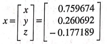
:. x=0.759674, y=0.260692 and z=−0.177189

Hence the least squares solution is

 

Example 6

Solve the following system of equations by using the method of least squares solution.

2x₁+2x₂−2x₃=1

2x₁+2x₂−2x₃=3

−2x₁2x₂+6x₃ = 2

Solution:

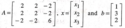
From the given system of equations, we have

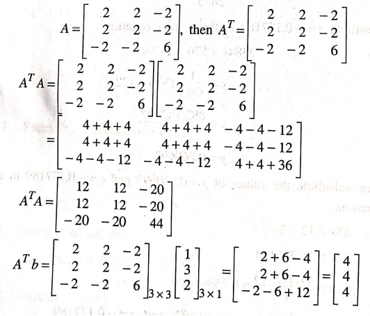
1. Compute A^TA and A^Tb

2. Form the augmented matrix

 A^TAx = A^Tb

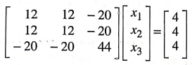
3. Method of solution:

Let AX=B             (Here A = A^TA)

where

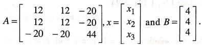
Let us apply Gauss elimination method to find the solution

((ie) Form the upper triangular matrix)

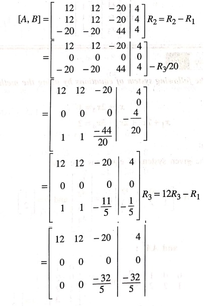
From the above matrix, by back substitution methods

12x₁ +12x₂−20x₃ = 4

 (−32/5) x₃ = −32 / 5

From the last equation x₃ = 1.

Put x₃ = 1 in the first equation, then 12x₁ +12x₂ = 4+20x₃

Therefore, 12x₁ + 12x₂ = 24

⇒ x₁=1 and x₂ = 1

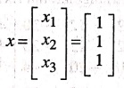
Hence the solution is x₁ = 1, x₂ = 1 and x₃ = 1.

The solution of the least squares solution is

 

Example 7

Solve the following system of equations by using the method of least squares.

 x₃+2x₄=1

 x₁+2x₂+2x₃+3x₄=2

Solution:

From the given system of equations, we have

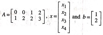
1. Compute A^T and AA^T:

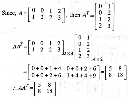
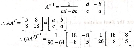
2. Calculate the inverse of AA^T:

 The inverse of a 2×2 matrix A =  is defined as

We can use Cayley−Hamilton theorem to find inverse.

  |AA^T – λI 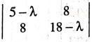| = 0

 = 0

⇒ (5 − λ) (18 − λ) ‒ 64 = 0

 90 − 5λ − 18λ + λ² −64 = 0

 λ² − 23λ + 26 = 0

 A² − 23A + 26I = 0

(÷ by A^‒1);

 Then A−23I+26A^‒1=0

 26A⁻¹ = [23I−A]

A⁻¹ = 1/26 [23I−A]              (where A = AA^T)

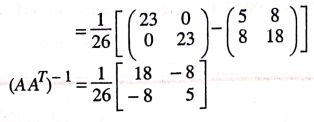
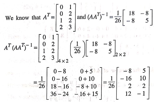
3. Calculate A^T(AA^T)⁻¹;

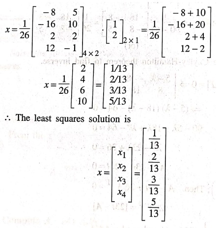
4. Calculate the final solution x = A^T(AA^T)^‒1.b:

 

Example 8

Find the least squares solution to the following system of equations.

x₁+x₂+3x₃ = 1

x₁+x₂+3x₃ = 2

Solution:

From the given system of equation, we have

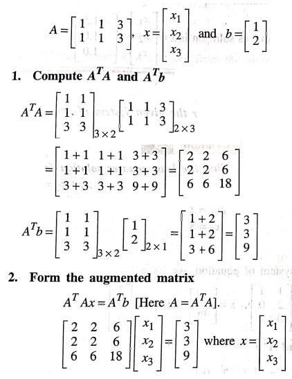
3. Method of solution

Let AX=B                [Here A = A^TA]

Let us apply Gauss elimination method to find the solution.

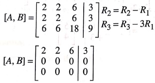
  The above matrix gives a single equation 2x₁ + 2x₂ + 6x₃ = 3.

(i.e.,) x₁+x₂+2x₃ = 1.5

This single equation has an infinite number of solutions. To express the general solution, we can introduce two free parameters, as x₂ = 1 and x₃ = 1.

Then x₁=1.5−x₂−2x₃ becomes x₁ = 1.5−1−2(1)

 x₁=1.5−3

 x=1.5

Hence the solution is x₁ = 1.5, x₂=1 and x₃ = 1.

The least squares solution is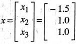  

 

Example 9

Find the least squares solution for the given system of equations.

x₁+x₂=1

2x₁=2

x₂=3

Solution:

From the given system of equation, we have

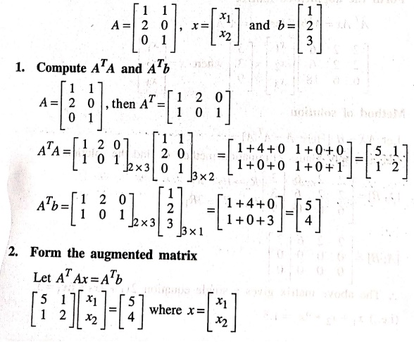
3. Method of solution

Let AX= B.                  (Here A = A^TA)

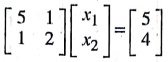
Let us apply Gauss elimination method to find solution.

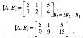
By using the back substitution method, from the above matrix,

 5x₁+x₂=5

 9x₂ = 15

⇒  x₂ = 15/9 = 5/3

Substitution x₂ = 5/3 in 5x₁ + x₂ = 5.

Then 5x₁ = 5 − x₂ = [5 - 5/3] = 10/3

x₁ = 1/5(10/3) = 2/3

x₁ = 2/3; and x₂ = 5/3.

 The least squares solution is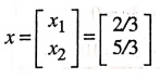  

 

Example 10

Find the least squares line y = mx +c that best fits the data points (0, 6), (1, 0) and (2, 0).

Solution:

From the above data, let us construct the value as

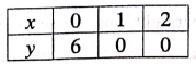
The data can be marked as in the following table.

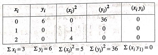
For this type of data problems, we have to use the following normal equations.

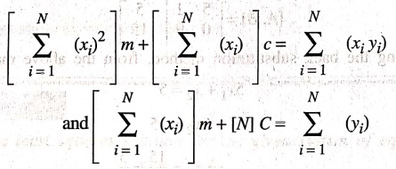
where N No. of the total data. (ie) N=3.

From the above two normal equations, we have

 5m+3c=0          ... (1)

 3m+3c=6          ... (2)

⇒ 5m+3c=0 and          ... (3)

 m+c=2          ... (4)

 (3):       5m+3c = 0

(4) × 5:  5m+5c = 10

(−)               ‒2c = ‒10

  ⇒     c=5.

Put c=5 in equation (4). Then we get m=2−c

m=2−5

 m=−3.

The values are m = −3 and c = 5.

 The least squares straight line y = mx + c becomes y = − 3x+5.

 

Example 11

Find the least squares straight line for the following xy data.

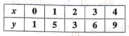
Solution:

From the above data, let us construct the following table.

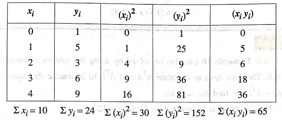
For this type of the problems, we have to use the following normal equations.

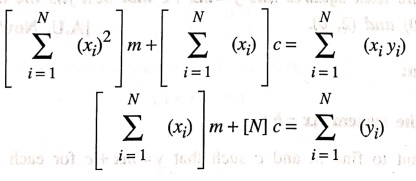
Here N represents the total number of data.

 (ie) N=5

From the above two equation ()

30m+10c = 65 and       ..... (1)

10m+5c=24             ... (2)

From (1):         30m + 10c = 65

From (2) × 3:   30m + 15c = 72

 (−)                              −5c = −7

    c = 7/5

From equation (2); 10m=24−5c

⇒ 10m=24−5(7/5)

 10m = 17 and hence m=17/10 = 1.7

Hence m = 1.7 and c = 1.4

  The least squares straight line y=mx+c becomes

y= (1.7)x+(1.4)

 

Note: Now Example 10 can also be solved by using the system of equation Ax=b. Then we have to calculate A^TA and A^Tb to formulate the equation A^TAx=A^Tb, to find the solution.

This method is illustrated in Example 12.

 

Example 12

Find the least squares line y=mx+c that best fits the data points (0, 6), (1, 0) and (2, 0).

Solution:

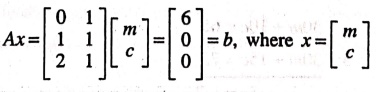
1. Form the system Ax=b:

We want to find m and c such that y=mx+c for each data point.

This gives the system.

For the point (0, 6): m(0) + c = 6)

For the point (1, 0): m(1)+c=0

For the point (2, 0): m (2)+c=0

This can be written in matrix form as

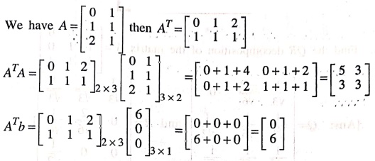
2. Calculate A^TA and A^Tb:

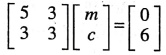
3. Solve the normal equations A^TAx = A^Tb:

  A^TAx = A^Tb

Let us apply the Gauss eliminating method to find m and c.

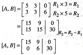
By using back substitution method, we have

15m+9c=0

6c = 30

⇒  c= 30/6 = 5.

Substitute c=5 in 15m+9c=0 then 15m=−9c

15m=−45

⇒ = −45/15

⇒ m = −3.

 m=−3 and c=5.

The least squares regression line is y = mx + c

 y = −3x+5