QR Decomposition: Example Solved Problems

QR Decomposition

WORKED EXAMPLES

 

Example 1

Use the modified Gram−Schmidt process to construct an orthogonal set of vectors from the linearly independent set { X₁, X₂, X₃ } where

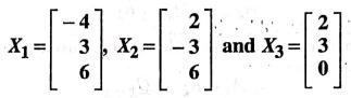
Solution:

First iteration

r₁₁ = || X₁ ||₂ = √ <X₁, X₁> = √[(− 4)² + (3)² + (6)²] = √[16+9+36] = √61.

 r₁₁= || X₁ ||₂ = 7.81025

 Q₁ = (1/r₁₁). X₁ = 1/7.81025 [−4, 3, 6]^T

= [ ‒4/7.81025 , 3/7.81025 , 6/7.81025 ]

Q₁ = [− 0.512148, 0.384111, 0.768221]^T

r₁₂ = <X₂, Q₁>

= < (2,−3, 6), (−0.512148, 0.384111, 0.768221) >

= [ (2)(− 0.512148) + (− 3)(0.384111) + (6)(0.768221) ]

= [−1.024296 − 1.152333 + 4.609326]

 r₁₂ = 2.432697

 r₁₃ = <X₃, Q₁>

= < (2, 3, 0), (−0.512148, 0.384111, 0.768221) >

= [(2) (−0.512148) + (3)(0.384111) + (0)(0.768221)]

= [−1.024296 + 1.152333 + 0]

 r₁₃=0.128037

X₂ = X₂ − r₁₂Q₁

= [2,−3, 6]^T − 2.432697[−0.512148, 0.384111, 0.768221]^T

= [2,−3, 6]^T + [1.2459,−0.934426, −1.86885]^T

X₂ = [3.2459, − 3.934426, 4.13115]^T

X₃ = X₃ − r₁₃Q₁

= [2, 3, 0]^T − (0.128037) [−0.512148, 0.384111, 0.768221]^T

= [2, 3, 0]^T + [0.06557,−0.04198, −0.09368]^T

X₃ = [2.06557, 2.95082−0.09836]^T

Second iteration: (from the first iteration data)

r₂₂ = || X₂ ||₂ = √ <X₂, X₂> = √[ (3.2459)² + (− 3.934426)² + (4.13115)²]

= √[ 10.53587 + 15.47971 + 17.06640 ] = √43.08198

 r₂₂ = 6.563686

Q₂ = (1/r₁₁). X₂ = 1/1 6.563686 [3.2459, 3.934426, 4.13115]^T

Q₂ = [0.494524, −0.599423, 0.629394]^T

 r₂₃ = <X₃, Q₂>

= < (2.06557, 2.95082,−0.09826), (0.494524, −0.599423, 0.629394) >

= [ (2.06557)(0.494524) + (2.95082)(−0.599423) + (−0.09836) (0.629394) ]

= [1.021473 − 1.768789 − 0.061907]

 r₂₃ = − 0.809223

 X₃ = X₃ − r₂₃Q₂

= [2.06557, 2.95082,−0.09836]^T + 0.809223[0.494524, −0.599423, 0.629394]^T

= [2.06557, 2.95082, − 0.09836]^T + [0.400181, −0.485067, 0.509321]^T

 X₃ = [2.465751, 2.465753, 0.410961]^T

Third iteration: (from the second iteration data)

 r₃₃ = || X₃ ||₂ = √[(2.465751)² + (2.465753)² + (0.410961)²]

= √[6.079927 +6.079937 +0.168888]

= √12.328752

 r₃₃ = 3.511232

 Q₃ = (1/r₃₃)X₃ = 1/3.511232 [2.465751, 2.465753, 0.410961]^T

Q₃ = [0.702246, 0.702247, 0.117041]^T

  An orthonormal set is {Q₁, Q₂, Q₃}

 

Example 2

Construct a QR decomposition for the given matrix

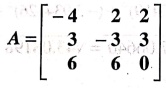
Solution:

We know that the QR decomposition is A = QR. Where A is the given matrix, Q is the matrix which consists of Q₁, Q₂, Q₃ (ie) [Q₁, Q₂ Q₃] and R is the upper triangular matrix in the form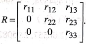  

From the Example 1, the given matrix A can be written as

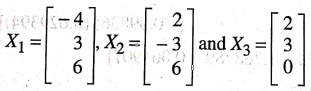
Then we have to apply modified Gram−Schmidt process to construct an orthogonal set of vectors from the linearly independent set {X₁, X₂, X₃} for the considered column vectors X₁, X₂, X₃.

From Example (1), we have

Q₁ = [−0.512148, 0.384111, 0.768221]^T

Q₂ = [0.494524, −0.599423, 0.629395]^T

Q₃ = [0.702247, 0.702247, 0.117041]^T

R = 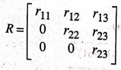 is an upper triangular matrix.

 From Q₁, Q₂ and Q₃ we can formulate the elements of Q and R.

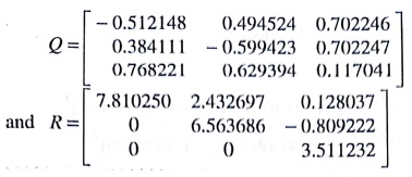
A direct calculation shows that A = QR.

 

Example 3

Construct a QR decomposition for the given matrix A = .

Solution:

We know that the QR decomposition is A = QR.

From the given matrix A, we have

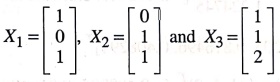
First iteration

 r₁₁ = || X₁ ||₂ = √<X₁, X₁> = √[1² +0² + 1²] = √2 = 1.414213.

 Q₁ = 1/(r₁₁) . X₁ = 1 / 1.414213 [1, 0, 1]^T

 Q₁ = [0.707107, 0.0, 0.707107]^T

 r₁₂ = <X₂, Q₁> = < (0, 1, 1), (0.707107, 0.0, 0.707107) >

 = [0 (0.707107) + 1 (0.0) + (1)(0.707107)] = [0+0+0.707107]

 r₁₂ = 0.707107

 r₁₃ = <X₃, Q₁> = < (1, 1, 2), (0.707107, 0.0, 0.707107) >

= [1 (0.707107) + 1 (0.0) + 2 (0.7071071)] = [0.707107+0+1.414214]

 r₁₃ = 2.121321

 X₂ = X₂−r₁₂Q₁

= [0, 1, 1]^T − 0.707107 [0.707107, 0.0, 0.707107]^T

= [0, 1, 1]^T + [−0.499947, 0.0, −0.499947]^T

 X₂ = [−0.499947, 1.0, 0.500053]^T

 X₃ = X₃−r₁₃Q₁

= [1, 1, 2]^T − 2.121321[0.707107, 0.0, 0.707107]^T

= [1, 1, 2]^T + [−1.5000009, 0.0,− 1.5000009]^T

X₃ = [−0.5000009, 1.0, 0.4999991]^T

Second iteration: (from the first iteration)

 r₂₂ = || X₂ ||₂ = √<X₂, X₂>

= √[(− 0.499947)² + (1.0)² + (0.500053)²]

= √[0.249947 + 1.0+ 0.250053] = √1.5

 r₂₂ = 1.224745

Q₂ = 1/(r₂₂) . X₂ = 1 / 1.224745 [‒0.499947, 1.0, 0.500053]^T

Q₂ = [−0.408205, 0.816496, 0.408291]^T

 r₂₃ = <X₃, Q₂> = < (1, 1, 2)^T, (−0.408205, 0.816496, 0.408291)^T >

= [ (1)(−0.408205) + (1)(0.816496) + (2)(0:408291) ]

= [−0.408205+0.816496 +0.816582]

 r₂₃ = 1.224873

X₃ = X₃−r₂₃Q₂

= [−0.5000009, 1.0, 0.4999991])^T − 1.224873[−0.408205, 0.816496, 0.408291]^T

= [−0.5000009, 1.0, 0.499999]^T + [0.499999,− 1.000103, −0.500105]^T

X₃ = [−0.0000019, −0.000103, −0.0001059]^T

Third iteration: (from the second iteration)

r₃₃= || X₃ ||₂ = √[(−0.0000019)² + (− 0.000103)² + (−0.0001059)²]

= √[0.00000000 +0.000000011 +0.0000001121]

=√0.00000002121

r₃₃ = 0.000149

Q₃ = 1/r₃₃ • X₃

= 1/0.000149 [−0.0000019, −0.000103, −0.0001059]^T

Q₃ = [−0.012837,−0.691275,−0.710738]^T

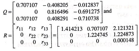
A direct calculation shows that A= QR.

 

Example 4

Construct the QR decomposition for the given matrix

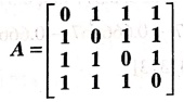
Solution:

Let us consider

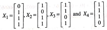
First iteration

We know that A = QR

Let r₁₁ = || X₁ ||₂ = √<X₁, X₁> = √[0² + 1² + 1² + 1²] = √3 = 1.732051

Q₁ = 1/r₁₁ . X₁ = 1/√3 [0, 1, 1, 1]^T = [ 0, 1/√3, 1/√3, 1/√3 ]^T

Q₁= [0, 0.577350, 0.577350, 0.577350]^T

r₁₁ = <X₂, Q₁>

= < (1, 0, 1, 1), (0, 0.577350, 0.577350, 0.577350) >

= [(1) 0+ (0) 0.577350+ (1) 0.577350+ (1) 0.577350]

= [0+0+0.577350 +0.577350]

r₁₂ = 1.1547

r₁₃ = <X₃, Q₁>

= < (1, 1, 0, 1), (0, 0.577350, 0.577350, 0.377350) >

= [1(0) + (1)0.577350 + (0)0.577350 + (1)0.577350]

= [0+0.577350+0+0.577350]

 r₁₃ = 1.1547

r₁₄ = < X₄,Q₁ >

= < (1, 1, 1, 0), (0, 0.577350, 0.577350, 0.577350) >

= [(1) 0+ (1) 0.577350 + (1) 0.57735 + (0) 0.577350]

= [0+0.577350+0.577350+0]

r₁₄ = 1.1547

X₂ = X₂−r₁₂Q₁

= [1, 0, 1, 1]^T ‒ 1.1547[0, 0.577350, 0.577350, 0.577350]^T

= [1, 0, 1, 1]^T + [0, − 0.666667, −0.666667, – 0.666667]^T

X₂ = [1, − 0.666667, 0.333333, 0.333333]^T

X₃ = X₃ − r₁₃Q₁

= [1, 1, 0, 1]^T – 1.1547[0, 0.577350, 0.577350, 0.577350]^T

= [1, 1, 0, 1]^T + [0, − 0.666667, − 0.666667, – 0.666667]^T

 X₃ = [1, 0.333333, – 0.666667, 0.333333]^T

X₄ = X₄ − r₁₄Q₁

= [1, 1, 1, 0]^T – 1.1547 [0, 0.577350, 0.577350, 0.577350]^T

= [1, 1, 1, 0]^T + [0, − 0.666667, −0.666667, – 0.666667]^T

X₄ = [1, 0.333333, 0.333333,− 0.666667]^T

Second iteration: (from the iteration vectors)

 r₂₂ = || X₂ ||₂ = √[(1)² + (−0.666667)² + (0.333333)² + (0.333333)²]

= √[ 1 +0.444444 +0.111111 + 0.111111]

= √1.666666

r₂₂ = 1.290994

Q₂ = 1/r₂₂ . X₂

 = 1/1.290994 [1, − 0.666667, 0.333333, 0.333333]^T

Q₂ = [0.774596, −0.516398, 0.258198, 0.258198]^T

r₂₃ = <X₃, Q₂>

= < (1, 0.333333,−0.666667, 0.333333)^T, (0.774596, −0.516398, 0.258198, 0.258198)^T >

= [ (1)(0.774596) + (0.333333)(−0.516398) + (−0.666667)(0.258198) + (0.333333)(0.258198) ]

= [0.774596 −0.172132−0.172132 +0.086065]

r₂₃ = 0.516397

r₂₄ = (X₄, Q₂)

= < (1, 0.333333, 0.333333, ‒ 0.666667)^T, (0.774596, – 0.516398, 0.258198, 0.258198)^T >

= [ (1) 0.774596 − (0.333333)(0.516398) + (0.333333) (0.258198) − (0.666667) (0.258198)]

= [0.774596−0.172132 +0.086065 − 0.172132]

 r₂₄ = 0.516397

 X₃ = X₃ − r₂₃Q₂

= [1, 0.333333, −0.666667, 0.333333]^T − 0.516397[0.774596 −0.516398, 0.258198, 0.258198]^T

= [1, 0.333333, −0.666667, 0.333333]^T + [−0.399999, 0.266665, −0.133332, −0.133332]^T

X₂ = [0.600001, 0.599998, −0.799999, 0.200001]^T

X₄ = X₄− r₂₄Q₂

= [1, 0.333333, 0.333333,−0.666667]^T −0.516397 [0.774596 −0.516398, 0.258198 0.258198]^T

= [1, 0.333333, 0.333333, −0.666667]^T + [−0.399999, 0.266666, −0.133332, −0.133332]^T

X₄ = [0.600001, 0.599999, 0.200001, −0.799999]^T

Third iteration: (using vectors from the second iteration)

r₃₃ = || X₃ ||₂ = √<X₃, X₃>

= √[(0.600001)² + (0.599999)² + (− 0.799999)² + (0.200001)²]

= √[0.360001 +0.359998 +0.639998 +0.0400004]

= √1.399997

r₃₃ = 1.183215

Q₃ = 1/r₃₃ . X₃

= 1/1.183215 [0.600001, 0.599998, −0.799999, 0.200001]^T

 Q₃ = [0.507093, 0.507091, −0.676123, 0.169031]^T

r₃₄ = <X₄, Q₃ >

= < (0.600001, 0.599999, 0.200001, −0.799999)^T, (0.507093, 0.507091, – 0.676123, 0.169031)^T >

= [(0.600001) (0.507093) + (0.599999) (0.507091) + (0.200001) (−0.676123) + (−0.799999) (0.169031)]

= [0.304256+0.304254−0.134246 −0.135224]

r₃₄ = 0.33904

X₄ = X₄ − r₃₄Q₃

= [0.600001, 0.59999, 0.200001,−0.799999]^T – 0.33904 [0.507093, 0.507091, −0.676123, 0.169031]^T

= [0.600001, 0.59999, 0.200001, −0.799999]^T + [−0.171924, −0.171924, 0.229232, −0.057308]^T

X₄ = [0.428077, 0.428075, 0.429233,−0.857307]^T

Fourth iteration: (using the vector from the third iteration)

 r₄₄ = || X₄ ||₂ = √[0.183249 +0.183248 +0.184241 +0.734975]

= √1.285713

r₄₄ = 1.133892

Q₄ = 1/r₄₄ . X₄

= 1/1.133892 [0.428077, 0.428075, 0.429233, −0.857307]^T

Q₄= [0.377528, 0.377527, 0.378548, −0.756074]^T

  The QR decomposition is

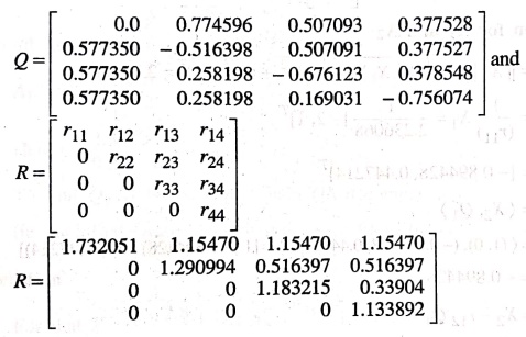
A direct calculation shows that A = QR.

 

Example 5

Apply the shifted QR algorithm to the matrix A =  to find the eigenvalues.

Solution:

We know that the shifted QR algorithm is

A_k−1 − S_k−1I = Q_k−1 R_k−1 and

A_k = R_k−1Q_k−1 + S_k−1I

Put k=1: The first equation becomes

 A₀ – S₀I = Q₀R₀

First iteration:

Let us consider A0 = , and S0 = 5

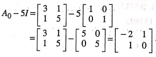
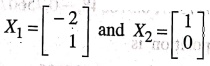
Now let us consider  We have to apply QR decomposition for this matrix by defining

I−iteration for X₁ and X₂

 r₁₁ = || X₁ ||₂ = √<X₁, X₁> = √(−2)² + (1)² = √5=2.236068

Q₁ = 1/(r₁₁) X₁ = 1/2.236068 [‒2,1]^T

Q₁ = [−0.894428, 0.447214]^T

 r₁₂ = <X₂, Q₁>

= < (1, 0), (−0.894428, 0.447214) >

= [1 (0.894428) + 0 (0.447214)]

r₁₂ = −0.894428

X₂ = X₂ − r₁₂Q₁

= [1,0]^T +0.894428[−0.894428, 0.447214]^T

= [1, 0]^T + [−0.800001, 0.400001]^T

X₂ = [0.199999, 0:4000011]^T

II−iteration

r₂₂ = ||X₂||₂ = √<X₂, X₂> =√[(0.199999)² + (0.400001)²]

= √[0.039999 +0.160001] = √0.2

 r₂₂ = 0.447214

Q₂ = 1/r₂₂ . X₂ = 1/0.447214 [0.199999, 0.40001]^T

Q₂ = [0.447191, 0.894429]^T

Here R₀ is the upper triangular matrix 

Now the second equation for the shifted QR algorithum is

 A₁ = R₀Q₀+ S₀l

A₁ = R₀Q₀ + 5I

Second iteration

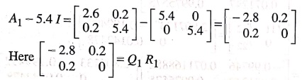
To find Q₁R₁ let us apply gain QR decomposition

(ie. modified Gram−Schmidt process to find Q₁R₁)

I−iteration

For that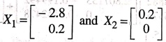  

 r₁₁ = || X₁ ||₂ = √ <X₁, X₂> = √[(− 2.8)² + (0.2)²] = √(7.84 + 0.04)

= √7.88 = 2.80713377

 r₁₁ = 2.807133

 Q₁ = 1/r₁₁ . X₁ = 1/2.807133 [−2.8, 0.2]^T

 Q₁= [−0.99746, 0.071247]^T

 r₁₂ = <X₂, Q₁> = < (0.2, 0), (− 0.99746, 0.071247) >

= [(0.2) (− 0.99746) + (0) (0.071247)] = −0.199492

X₂ = X₂ − r₁₂Q₁

= [0.2, 0]^T + 0.199492[−0.99746, 0.071247]^T

= [0.2, 0]^T + [−0.198986, 0.014213]^T

X₂ = [0.001014, 0.014213]^T

II−iteration

 r₂₂= || X₂ ||₂ = √[(0.001014)² + (0.014213)²]

= √[0.000001028 +0.000202001]

= √0.000203037 = 0.0142478

 r₂₂ = 0.0142478

Q₂ = 1/r₂₂ . X₂ = 1/0.0142478 [0.001014, 0.014213]^T

Q₂ = [0.71168882, 0.9975575]^T

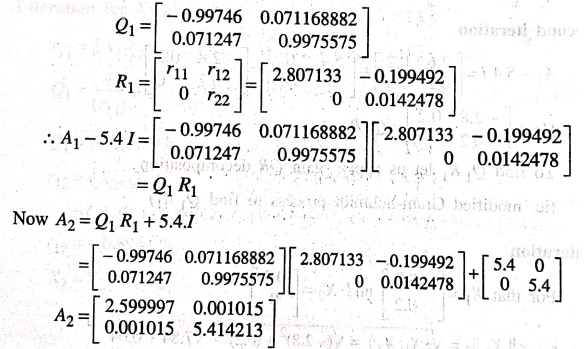
Third iteration:

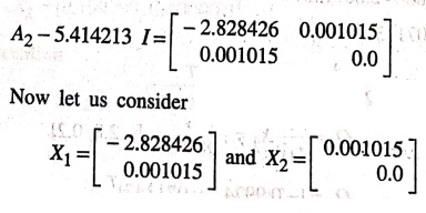
Let us apply modified Gram−Schmidt process to construct QR decomposition for the above X₁ and X₂.

After applying the Gram−Schimdt process, we get

 Q₁ = [−1.0, 0.000359]^T and Q₂ = [0.000359, 1.0]^T

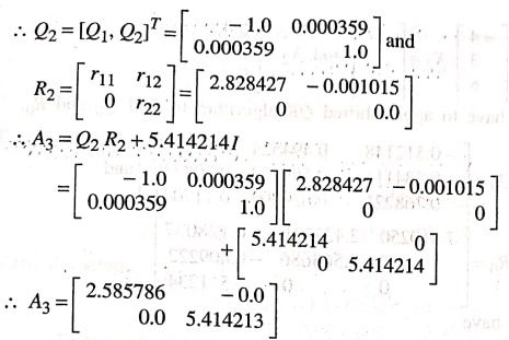
 The eigenvalues of A₃ are

 λ₁ = 2.585786 and λ₂ = 5.414213

 

Example 6

Apply shifted QR algorithm to A=  and find the eigenvalues.

Solution:

Let us consider A₀ =  

We know that the shifted QR algorithm is

A_k−1 − S_k−1I = Q_k−1R_k−1 and

A_k = R_k−1Q_k−1 + S_k−1I

Put k = 1; the first equation becomes A₀−S₀I = Q₀R₀

First iteration:

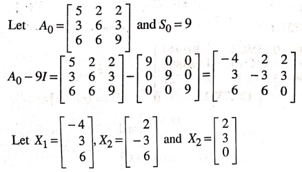
Now we have to apply shifted QR algorithm to find Q₀ and R₀.

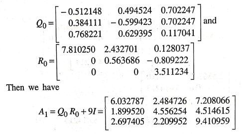
Second iteration:

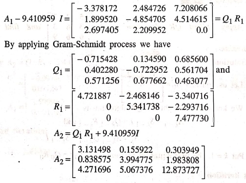
By applying Gram−Schmidt process we have

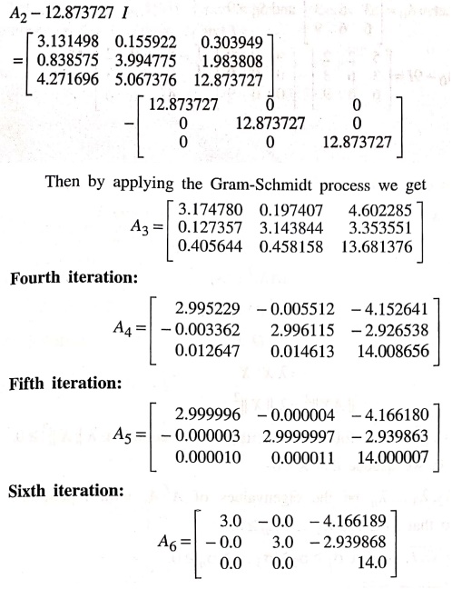
 The three eigenvalues are 3, 3, 14.0