Singular Value Decomposition: Example Solved Problems

SINGULAR VALUE DECOMPOSITION

WORKED EXAMPLES

 

Example 1

Determine the singular value decomposition for the matrix .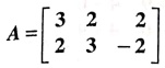

Solution:

Step 1: Compute AA^T

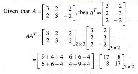
Step 2: Find the eigenvalues of AA^T

From step 1. We have AA^T = 

The characteristic polynomial is [AA^T — λI] = 0

|AA^T — λI| = 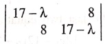 = 0

 (17−λ)²−64−0

289 + λ² – 34λ− 64 = 0

=> λ² ‒ 34λ + 225 = 0

 (λ−9)(λ−25) = 0

 The eigenvalues are λ = 25, 9.

Hence the eigenvalues are λ₁ = 25 and λ₂ = 9. These eigenvalues correspond to the singular values σ₁ = √λ₁ = √25 = 5 and σ₂ = √λ₂ = √9 = 3, since the singular values are the square roots of these eigenvalues.

Step 3: Find the right singular vectors (Eigenvectors of A^TA)

Now we find the eigenvectors of A^TA for λ₁ = 25 and λ₂ = 9.

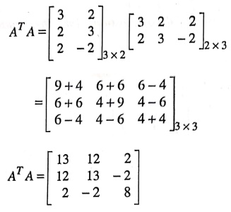
Case (i): When λ=25, then the eigenvector is [A^TA− λI]V=0

 (ie) [A^TA – 25I] V = 0 where 

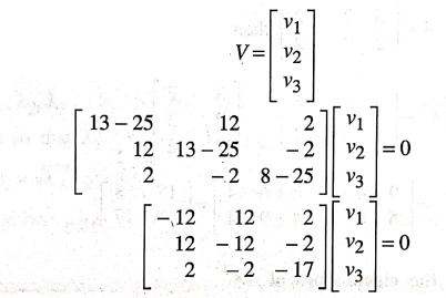
 −12v₁+12v₂−2v₃ = 0

12v₁−12v₂−2v₃=0

2v₁−2v₂−17v₃=0

Let us consider the last two equations

12v₁−12v₂−2v₃=0

2v₁−2v₂−17v₃=0

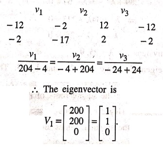
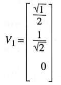
 The normalized form of the eigenvector corresponding to λ=25 is

Case (ii): When λ=9, the eigenvector is (A^TA−λI)V = 0

(ie) [A^TA – 9I]V = 0

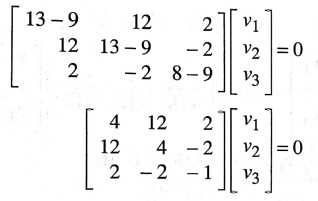
4v₁+12v₂+2v₃=0

12v₁+4v₂−2v₃=0

2v₁−2v₂ − v₃ = 0

Let us consider the first two equations

4v₁ + 12v₂ + 2v₃ = 0

12v₁ +4v₂ − 2v₃ = 0

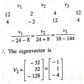
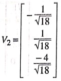
The normalized form of the eigenvector corresponding to λ=9 is

To find the third eigenvector V₃ :

Since V₃ must be perpendicular to V₁ and V₂, we solve the system V^T₁V₃ = 0 and V^T₂V₃ = 0.

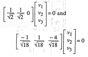
By solving these two equations we have

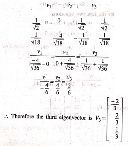
Therefore the corresponding third normalized form of eigenvector is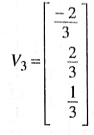

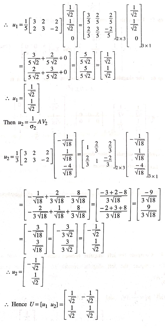
Step 4: Compute the left singular vectors (matrix U)

To compute the left singular vectors U, we use the formula u_i = 1/σ_i = AV_i.

u1 = 1/σ1 = AV1

u2 = 1/σ2 = AV2

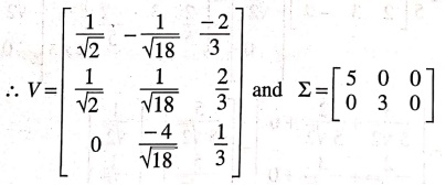
Step 5: Formulate the matrices V= [v₁ v₂ v₃] and Σ

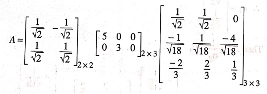
Step 6: The singular value decomposition of the matrix A is

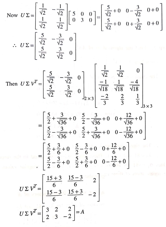
  A = UΣV^T

To verify the singular value decomposition

Let us verify the statement A=UΣV^T

 

Example 2

Find the singular value decomposition of the matrix A = .

Solution:

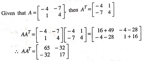
Step 1: Compute AA^T

Step 2: Find the eigenvalues of AA^T

From Step 1.

 AAT=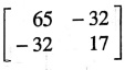

The characteristic polynomial is |AA^T−λI|=0

  |AAT−λI|=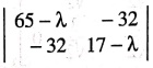=0

 (65−λ) (17− λ)−1024 = 0

1105 − 65λ − 17λ + λ² – 1024 = 0

λ²−82λ+81=0

 (λ−1)(λ−81)=0

The eigenvalues are λ=81 and 1.

 λ₁=81 and λ₂=1. These eigenvalues correspond to the singular values σ₁ = √81 = 9 and σ₂ = √λ₂ = √1 = 1, since the singular values are the square roots of these eigenvalues.

Step 3: Find the right singular vectors (Eigenvectors of A^TA)

Now we find the eigenvectors of A^TA for λ₁=81 and λ₂ = 1.

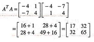
Case (i): When λ=81, the eigenvector is [A^TA−81I]V=0

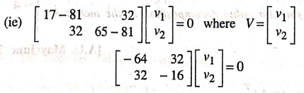
 −64v₁ + 32v₂ = 0

 32v₁−16v₂ = 0

By solving these two equations, we have

 −2v₁ + v₂ = 0

 2v₁−v₂ = 0

We have a single equation

2v₁−v₂=0

⇒ 2v₁ = v₂

Put v₁ =1 then v₂ = 2.

The eigenvector is V₁ = 

The normalized form of this eigenvector is V₁ =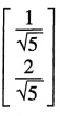 

Case (ii): When λ=1, the eigenvector is (A^TA − λI)V = 0

 [A^TA−1I] V=0

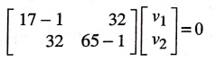
 16v₁+ 32v₂ = 0

 32v₁ +64v₂ = 0

  We have only one equation v₁ + 2v₂ =

 v₁ = −2v₂

Let us put v₁ = 1, then v₂ = ‒1⁄2

The eigenvector when λ=1 is v₂ =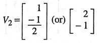 

The normalized form of the eigenvector is V₂ =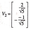 

Step 4: Compute the left singular vectors (matrix U)

To compute the left singular vectors U, we use the formula

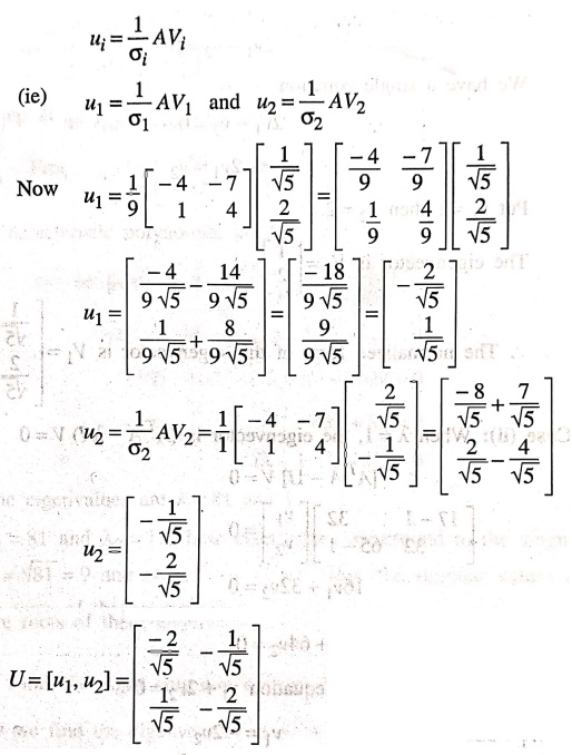
Step 5: Formulate the matrices V= [v₁, v₂] and Σ

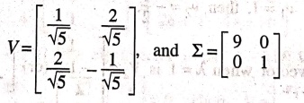
Step 6: The singular value decomposition is A = UΣV^T

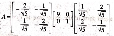
To verify the singular value decomposition

Let us verify the statement A= UΣV^T.

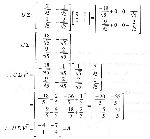
  The singular value decomposition is verified.

 

Example 3

Determine the singular value decomposition of the matrix A= 

Solution:

Step 1: Compute A^TA

Given that A= 

Step 2: Find the eigenvalues of A^TA

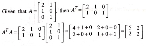
The characteristic polynomial is |A^TA−λI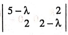| = 0.

 = 0

(5−λ) (2−λ)−4=0

10−5λ−2λ+λ²=0

λ² ‒ 7λ+6=0

 (λ−6) (λ−1)=0

  The eigenvalues are λ₁=6 and λ₂=1.

These eigenvalues correspond to the singular values

 σ₁ =√λ₁ = √6 and σ₂ = √λ₂ = √1=1, since the singular values are the square roots of eigenvalues.

Step 3: Find the right singular vectors (Eigenvectors of A^TA)

The eigenvector for the matrix [A^TA−λI]V=0

Case (i): When λ=6; the eigenvector is determined by

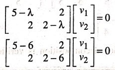
 −v₁+2v₂ = 0 and 2v₁−4v₂=0

Here we have a single equation v₁−2v₂=0

 v₁ = 2v₂

Let us consider v₁ =2 then v₂ = 1.

 The eigenvector when λ=6 is V₁ = 

The normalized form of eigenvector is V₁ =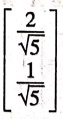 

Case (ii): When λ= 1; the corresponding equations are

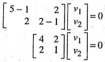
 4v₁+2v₂ = 0 and 2v₁+v₂=0.

Here also we have a single equation 2v₁+v₂=0

 2v₁ = ‒v₂

Put v₁ =1 then v₂ = −2.

.. The eigenvector when λ=1 is V₂ = 

The normalized form of V₂ is V₂ =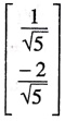 

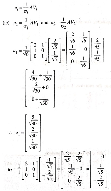
Step 4: Compute the left singular vectors (matrix U)

The compute the left singular vectors U₁ we use the formula

To find the remaining eigenvector

Let us consider A^TV=0

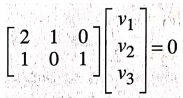
 2v₁+ v₂+0v₃ = 0

 1v₁ + 0v₂+ 1v₃ = 0

⇒ 2u₁+v₂ =0 and v₁+v₃=0

Put v₁ =1 then v₂=−2 and v₃ = − 1.

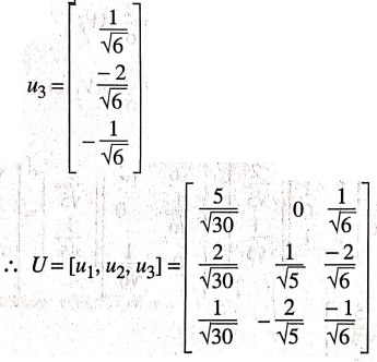
 The corresponding eigenvector is u₃ = 

  The corresponding normalized form is 

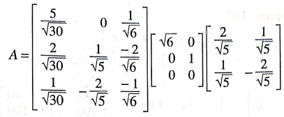
Step 6: Formulate the matrices V= [v₁, v₂] and Σ

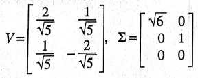
The singular value decomposition of the matrix A is A = UΣ V^T

To verify the singular value decomposition

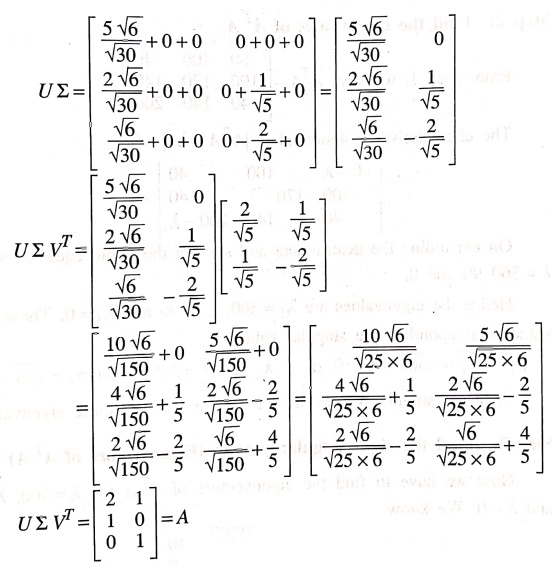
Let us verify the statement A=UΣV^T

 

Example 4

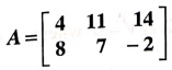
Find a singular value decomposition of the matrix

Solution:

Step 1: Compute AA^T

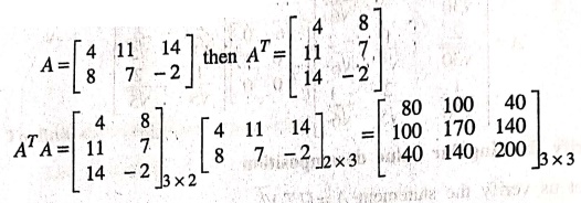
Step 2: Find the eigenvalues of A^TA

From Step 1, we have A^TA =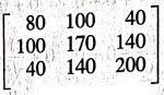 

The characteristic polynomial is |A^TA−λI|=0

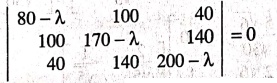
On expanding the determinant and solving the cubic equation we get λ=360, 90 and 0.

Hence the eigenvalues are λ₁=360, λ₂=90 and λ₃=0. These eigen values correspond to the singular values

σ₁ = √λ₁ = √360 = 6√10, σ₂ = √λ₂ = √90 = 3√10 and σ₃ = √λ₃ = 0,

since the singular values are the square roots of these eigenvalues.

Step 3: Find the right singular vectors (Eigenvectors of A^TA)

Now we have to find the eigenvectors of A^TA for λ=360, λ = 90 and λ=0. We know that, from step 1

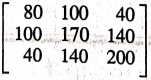
Case (i): When λ=360, then the eigenvector is

[A^TA−λI]V=0 where 

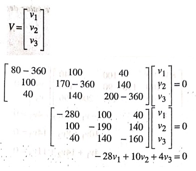
−28v₁ +10v₂ + 4v₃=0

10v₁−19v₂+14v₃=0

4v₁ +14v₂−16v₃=0

By solving the last two equations we have

 10v₁−19v₂+14v₃ = 0

 4v₁ + 14v₂ – 16v₃ = 0

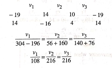
The eigenvector when λ=360 is V₁ = 

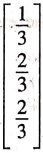
 The normalized form of V₁ is V₁ = 

Case (ii): When λ=90, the eigenvector is [A^TA−90I]V=0

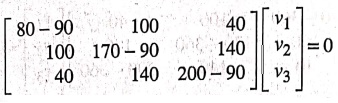
 −v₁+10v₂ + 4v₃ = 0

 10v₁ +8v₂ + 14v₃ = 0

 4v₁ + 14v₂ + 11v₃ = 0

By solving the first two equations,

 v₁ + 10v₂ + 4v₃ = 0

 10v₁ + 8v₂ + 14v₃ = 0

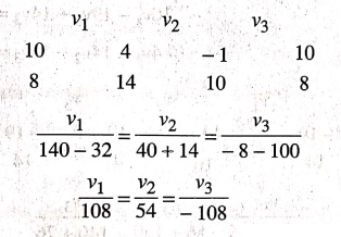
 The eigenvector when λ=90 is V₂ = 

The normalized form of V₂ is V₂ = 

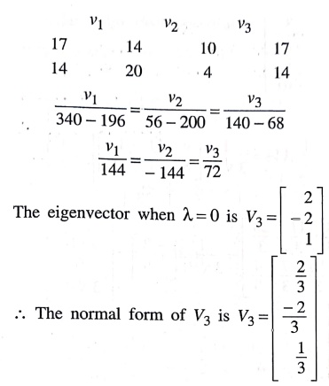
Case (iii): When λ=0, the eigenvector is [A^TA−0I] V=0.

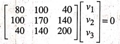
8v₁+10v₂+4v₃=0

10v₁ + 17v₂+14v₃=0

4v₁ + 14v₂+20v₃=0

Solving the last two equations

10v₁ + 17v₂+14v₃ = 0

4v₁ + 14v₂ +20v₃ = 0

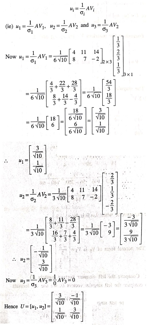
Step 4: Compute the left singular vectors (matrix U)

To compute the left singular vectors U, we use the formula

Step 5: Formulate the matrices V= [v₁, v₂, v₃] and Σ

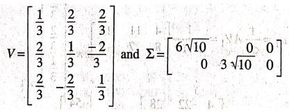
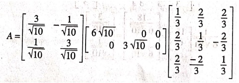
Step 6: The singular value decomposition of the matrix is

 A = UΣV^T

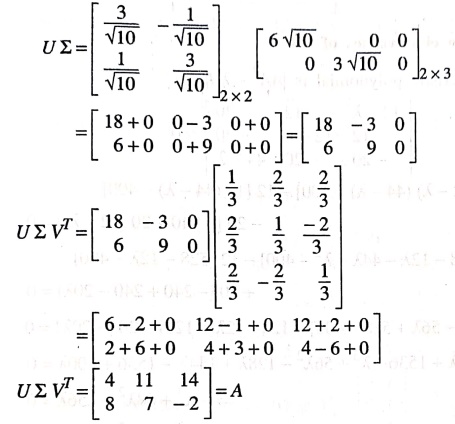
To verify the singular value decomposition

We can verify the statement A = UΣV^T.

 

Example 5

Determine the singular value decomposition for the matrix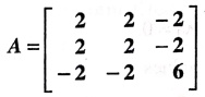 

Solution:

Step 1: Compute AA^T

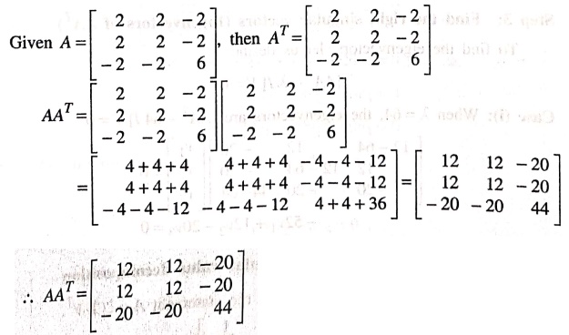
Step 2: Find the eigenvalues of AA^T

The characteristic polynomial is |AA^T−λI| = 0

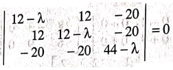
 (12−λ) [(12−λ) (44−λ)−400]−12[12 (44−λ)−400] − 20 [−240+20 (12 − λ)] = 0

(12− λ) [528−12λ −44λ + λ²−400]−12 [528−12λ −400] − 20 [−240+240−20λ]=0

(12 – λ) [λ² – 56λ + 528−400] − 12[− 12λ +128] −20 [−20λ] = 0

12λ² − 672λ + 1536− λ³ + 56λ²−128λ + 144λ − 1536 + 400λ = 0

− λ³+68λ²−256λ = 0

 λ³ − 68λ² + 256λ = 0

(λ ‒ 0) (λ ‒ 64) (λ − 4) = 0

 The eigenvalues are λ = 64, 4, 0.

Hence the eigenvalues are λ₁ = 64, λ₂=4 and λ₃ = 0.

These eigen values correspond to the singular values

 σ₁ =√λ₁ = √64 =8, σ₂ = √λ₂ = √4 = 2 and σ₃=0.

since the singular values are the square roots of these eigenvalues.

Step 3: Find the right singular vectors (Eigenvectors of AA^T)

To find the eigenvectors, let us define

 [AA^T – λI]V = 0

Case (i): When λ=64, the eigenvectors are [AA^T − 64I]V=0

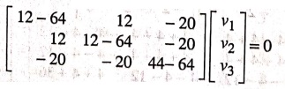
 −52v₁ + 12v₂ − 20v₃ = 0

12v₁−52v₂−20v₃ = 0

−20v₁−20v₂−20v₃=0

On simplification, we have

 −13v₁ +3v₂−5v₃=0

 3v₁−13v₂−5v₃ = 0

 −5v₁−5v₂−5v₃ = 0

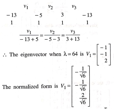
To solve these equation let us consider the last two equations,

 3v₁−13v₂−5v₃ = 0

 v₁+v₂ + v₃ = 0

Case (ii): When λ=4, the eigenvectors are [AA^T – 4I] V=0

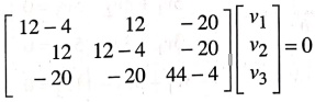
8v₁ + 12v₂ – 20v₃ = 0

12v₁+8v₂−20v₃=0

−20v₁−20v₂+40v₃=0

On simplifying, we have

2v₁ +3v₂−5v₃=0

3v₁ +2v₂−5v₃=0

v₁+v₂−2v₃=0

Consider the first two equations, we have

 2v₁ +3v₂−5v₃=0

 3v₁+2v₂−5v₃=0

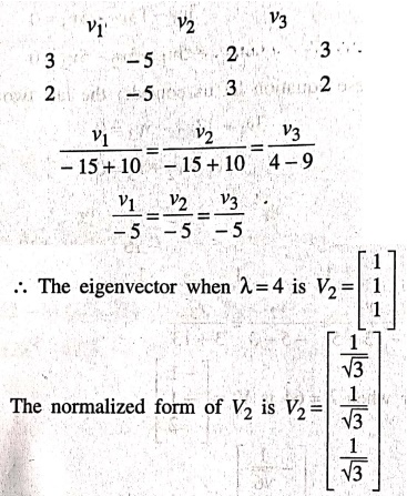
 The eigenvector when λ=4 is V₂

The normalized form of V₂ is V₂

Case (iii): When λ=0, the eigenvectors is [AA^T−0I] V=0

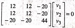
3v₁ +3v₂−5v₃=0

3v₁+3v₂−5v₃=0

−5v₁−5v₂−11v₃=0

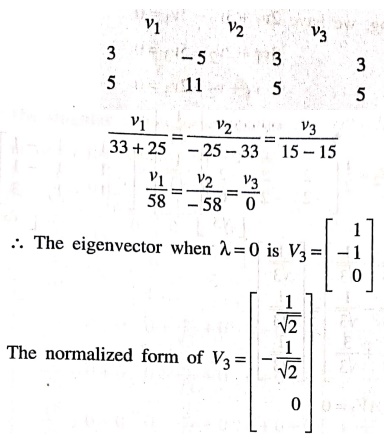
By considering the last equations, we have

3v₁ +3v₂−5v₃=0

5v₁ +5v₂ + 11v₃=0

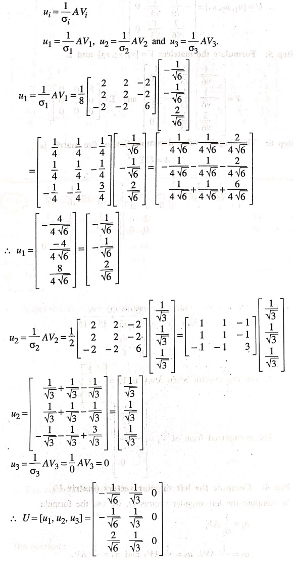
 Step 4: Compute the left singular vectors (matrix U)

To compute the left singular vectors U, we use the formula

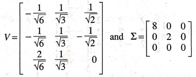
Step 5: Formulate the matrices V = [v₁, v₂, v₃] and Σ

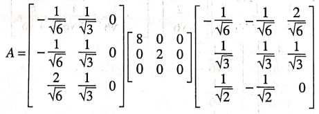
Step 6: The singular value decomposition of the matrix is

A=UΣV^T

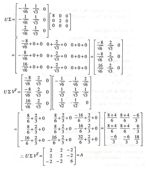
To verify the singular value decomposition

We can verify the statement A = UΣV^T.