Digital Storage Oscilloscope

DIGITAL STORAGE OSCILLOSCOPE

The digital storage oscilloscope is an instrument which gives the storage of a digital waveform or the digital copy of the waveform. It allows us to store the signal or the waveform in the digital format, and in the digital memory also it allows us to do the digital signal processing techniques over that signal. The maximum frequency measured on the digital signal oscilloscope depends upon two things they are: sampling rate of the scope and the nature of the converter. The traces in DSO are bright, highly defined, and displayed within seconds.

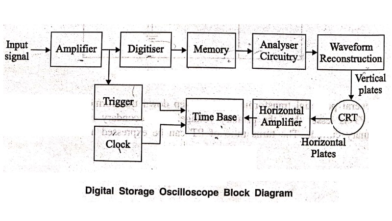
Block Diagram of Digital Storage Oscilloscope

The block diagram of the digital storage oscilloscope consists of an amplifier, digitizer, memory, analyzer circuitry. Waveform reconstruction, vertical plates, horizontal plates, cathode ray tube (CRT), horizontal amplifier, time base circuitry, trigger, and clock. The block diagram of the digital storage oscilloscope is shown in the figure 6.28.

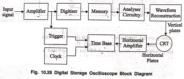
As seen in the above figure, at first digital storage oscilloscope digitizes the analog input signal, then the analog input signal is amplified by amplifier if it has any weak signal. After amplification, the signal is digitized by the digitizer and that digitized signal stores in memory. The analyzer circuit process the digital signal after that the waveform is reconstructed (again the digital signal is converted into an analog form) and then that signal is applied to vertical plates of the cathode ray tube (CRT).

The cathode ray tube has two inputs they are vertical input and horizontal input. The vertical input signal is the 'Y' axis and the horizontal input signal is the 'X' axis. The time base circuit is triggered by the trigger and clock input signal, so it is going to generate the time base signal which is a ramp signal. Then the ramp signal is amplified by the horizontal amplifier, and this horizontal amplifier will provide input to the horizontal plate. On the CRT screen, we will get the waveform of the input signal versus time.

The digitizing occurs by taking a sample of the input waveform at periodic intervals. At the periodic time interval means, when half of the time cycle is completed then we are taking the samples of the signal. The process of digitizing or sampling should follow the sampling theorem.

The sampling theorem says that the rate at which the samples are taken should be greater than twice the highest frequency present in the input signal. When the analog signal is not properly converted into digital then there occurs an aliasing effect.

When the analog signal is properly converted into digital then the resolution of the A/D converter will be decreased. When the input signals stored in analog store registers can be read out at a much slower rate by the A/D converter, then the digital output of the A/D converter stored in the digital store, and it allows operation up to 100 mega samples per second. This is the working principle of a digital storage oscilloscope.

Many different input channels are used with digital storage oscilloscopes. However if all these channels share a common store, through a multiplexer, then the memory available to each channel is reduced. Digital storage oscilloscopes with up to 40 channels are commercially obtainable, with a storage capability of 25000 dots. Several oscilloscopes also have floppy disc storage capability to allow non volatile storage of waveforms, which can later be recalled into the oscilloscope and manipulated.

DSO Operation Modes

The digital storage oscilloscope works in three modes of operations they are roll mode, store mode, and hold or save mode.

Roll Mode: In roll mode, very fast varying signals are displayed on the display screen.

Store Mode: In the store mode the signals stores in memory.

Hold or Save Mode: In hold or save mode, some part of the signal will hold for some time and then they will be stored in memory.

These are the three modes of digital storage oscilloscope operation.

Waveform Reconstruction

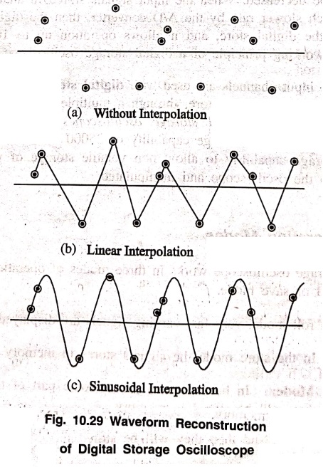
Although the input signal may be sampled at greater than twice the highest signal frequency, aliasing can still result when the output is present as a series of dots, corresponding to the sampled values. This is illustrated in the figure 6.29 (a) below, where the user's mind connects together the dots which are physically closest to each other, rather than those which are closest on the time scale.

In the illustration of the figure 6.29 (a), it is difficult to visualise the final waveform. And digital storage oscilloscopes generally have the facility to interpolate between the dots, if required by the user. Two techniques are used,

(i) Linear interpolation

(ii) Sinusoidal interpolation

Linear Interpolation: In linear interpolation, the dots are joined by a straight line.

Sinusoidal Interpolation: In sinusoidal interpolation, the dots are joined by a sine wave.

In linear interpolation, shown in the figure 6.29 (b) a straight line is used to connect the dots together. This works well on a pulsed or square waveform, but not on a sinusoidal wave, the figure 6.29 (c) shows that sinusoidal interpolation gives a much better fit for sine waves, although it is not suitable for pulse or square waves.

Another problem with the sampling technique used in digital storage oscilloscopes is that it can miss short term transient, or 'glitches', which occur in between the sample points. To overcome this problem envelope mode oscilloscopes may be used. These have special logic circuitry which causes the sample and digitising circuitry to run at a high speed, independent of the setting of the display time.

At each sample the value is compared with the previous stored sample, and the higher for lower) value is stored. This is continued for the screen interval, to that for that interval the highest and lowest points are always stored. For example, suppose that an oscilloscope digitises every 2 ms, at a given sweep speed.

If a 0.1 ms transient were to occur there is a high probability that a conventional digital storage oscilloscope would miss it.

In an envelope mode digital storage oscilloscopes, the input would be sampled, say, every 200 ns, but only the highest, or lowest, values that occur within a 2 ms window would be stored in memory. Therefore the transient would be recorded. The sample rate of the oscilloscope is controlled by the time setting of the oscilloscope, but the analog to digital converter runs very faster.