Handling Control Hazards

Handling Control Hazards

1. Instruction Queue and Prefetching

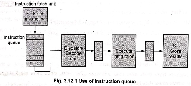
• To reduce the effect of cache miss or branch penalty, many processors employ sophisticated fetch units that can fetch instructions before they are needed and put them in a queue. This is illustrated in Fig. 3.12.1.

• A separate unit called dispatch unit takes instructions from the front of the queue and sends them to execution unit. It also performs the decoding function.

• The fetch unit attempts to keep the instruction queue filled at all times to reduce the impact of occasional delays when fetching instructions during cache miss.

• In case of data hazard, the dispatch unit is not able to issue instructions from the instruction queue. However, the fetch unit continues to fetch instructions and add them to the queue.

Use of instruction queue during branch instruction

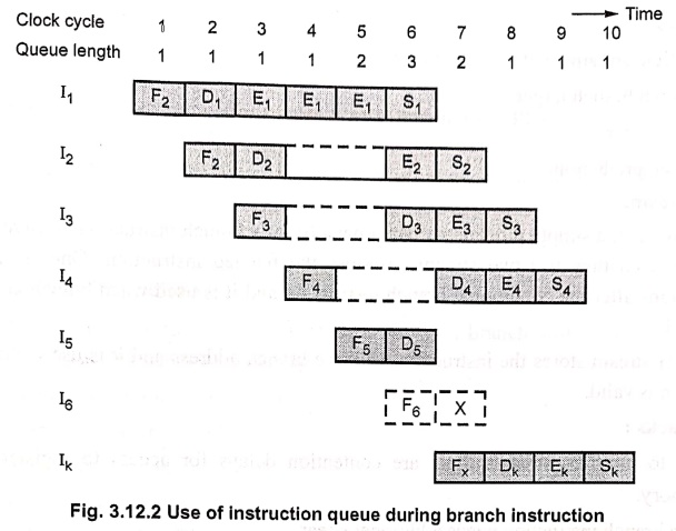
• Fig. 3.12.2 shows instruction time line. It also shows how the queue length changes over the clock cycles. Every fetch operation adds one instruction to the queue and every dispatch unit operation reduces the queue length by one. Hence, the queue length remains the same for the first four clock cycles.

• The instruction I₁ has 2‒cycle stall. In these two cycles fetch unit adds two instructions but dispatch unit does not issue any instruction. Due to this, the queue length rises to 3 in clock cycle 6.

• Since I₅ is a branch instruction, instruction I₆ is discarded and the target instruction of I₅ ,I_k is fetched in cycle 7. Since I is discarded, normally there would be stall in cycle 7; however, here instruction I₄ is dispatched from the queue to the decoding stage.

• After discarding I₆, the queue length drops to 1 in cycle 8. The queue length remains one until another stall is encountered. In this example, instructions I₁,I₂, I₃, I₄ and I_k complete execution in successive clock cycles. Hence, the branch instruction does not increase the overall execution time.

Branch folding

• The technique in which instruction fetch unit executes the branch instruction (by computing the branch address) concurrently with the execution of other instructions is called branch folding.

• Branch folding occurs only if there exists at least one instruction in the queue other than the branch instruction, at the time a branch instruction is encountered.

• In case of cache miss, the dispatch unit can send instructions for execution as long as the instruction queue is not empty. Thus, instruction queue also prevents the delay that may occur due to cache miss.

2. Approaches to Deal

• The conditional branching is a major factor that affects the performance of instruction pipelining. There are several approaches to deal with conditional branching.

• These are:

■ Multiple streams

■ Prefetch branch target

■ Loop buffer

■ Branch prediction.

1. Multiple streams

• We know that, a simple pipeline suffers a penalty for a branch instruction. To avoid this, in this approach they use two streams to store the fetched instruction. One stream stores instructions after the conditional branch instruction and it is used when branch condition is not valid.

• The other stream stores the instruction from the branch address and it is used when branch condition is valid.

• Drawbacks:

■ Due to multiple streams there are contention delays for access to registers and to memory.

■ Each branch instruction needs additional stream.

2. Prefetch branch target

• In this approach, when a conditional branch is recognized, the target of the branch is prefetched, in addition to the instruction following the branch. This already fetched target is used when branch is valid.

3. Loop buffer

• A loop buffer is a small very high speed memory. It is used to store recently prefetched instructions in sequence. If conditional branch is valid, the hardware first checks whether the branch target is within the buffer. If so, the next instructions are fetched from the buffer, instead of memory avoiding memory access.

Advantages:

■ In case of conditional branch, instructions are fetched from the buffer saving memory access time. This is useful for loop sequences.

■ If a branch occurs to a target just a few locations ahead of the address of the branch instruction, we may find target in the buffer. This is useful for IF‒THEN‒ELSE‒ENDIF sequences.

4. Delayed branch

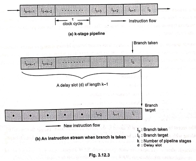
• The location following a branch instruction is called a branch delay slot. There may more than one branch delay slot, depending on the time it takes to execute a branch There may be instruction.

• There are three ways to fill the delay slot:

1. The delay slot is filled with an independent instruction before branch. In this case performance always improves.

2. The delay slot is filled from the target branch instructions. Performance improves if only branch is taken.

3. The delay slot is filled with an instruction which is one of the fall through instruction. In this case performance improves if branch is not taken.

• These above techniques are called delayed branching.

3. Branch Prediction

• Prediction techniques can be used to check whether a branch will be valid or not valid. These techniques reduce the branch penalty.

• The common prediction techniques are :

■ Predict never taken

■ Predict always taken

■ Predict by opcode

■ Taken/Not taken switch

■ Branch history table

• In the first two approaches if prediction is wrong a page fault or protection violation error occurs. The processor then halts prefetching and fetches the instruction from the desired address.

• In the third prediction technique, the prediction decision is based on the opcode of the branch instruction. The processor assumes that the branch will be taken from certain branch opcodes and not for others.

• The fourth and fifth prediction techniques are dynamic; they depend on the execution history of the previously executed conditional branch instruction.

Branch prediction strategies

• There are two types of branch prediction strategies :

■ Static branch strategy.

■ Dynamic branch strategy.

Static branch strategy: In this strategy branch can be predicted based on branch code types statically. This means that the probability of branch with respect to a particular branch instruction type is used to predict the branch. This branch strategy may not produce accurate results every time.

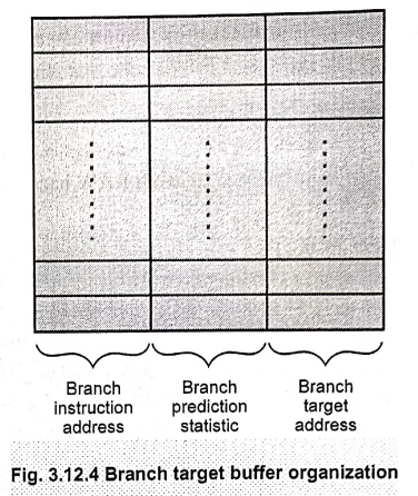
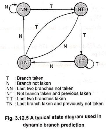
Dynamic branch strategy: This strategy uses recent branch history during program execution to predict whether or not the branch will be taken next time when it occurs. It uses recent branch information to predict the next branch. The recent branch information includes branch prediction statistics such as:

T : Branch taken

N : Not taken

NN : Last two branches not taken

NT : Not branch taken and previous takes

TT : Both last two branch taken

TN : Last branch taken and previous not taken

• The recent branch information is stored in the buffer called Branch Target Buffer (BTB).

• Along with above information branch target buffer also stores the address of branch target.

• Fig. 3.12.4 shows the organization of branch target buffer.

• Fig. 3.12.5 shows a typical state diagram used in dynamic branch prediction.

• This state diagram allows the backtracking of last two instructions in a given program. The branch target buffer entry contains the backtracking information which guides the prediction.

• The prediction information is updated upon completion of the current branch.

• To make branch overhead zero, the branch target buffer is extended to store the target instruction itself and a few of its successor instructions. This allows processing of conditional branches with zero delay.

Example: 1

The following sequence of instructions are executed in the basic 5‒stage pipelined processor :

lw$1, 40($6)

add $6, $2, $2

sw $6, 50($1)

Indicate dependence and their type. Assuming there is no forwarding in this pipelined processor, indicate hazards and add NOP instructions to eliminate them.

Solution:

a) I1: 1w $1, 40($6): Raw dependency on $1 from I1 to I3

I2: add $6, $2, $2: Raw dependency on $6 from I2 to I3

I3: sw $6,50 ($1) : WAR dependancy on $6 from I1 to I2 and I3

b) In the basic five‒stage pipeline WAR dependency does not cause any hazards. Assuming there is no forwarding in this pipelined processor RAW dependencies cause hazards – if register read happens in the second half of the clock cycle and the register write happens in the first half. The code that eliminates these hazards by inserting nop instruction is:

1w $1, 40($6)

add $6, $2, $2

nop; delay 13 to avoid RAW hazard on $1 from I1

sw $6,50($1)

Example: 2

A processor has five individual stages, namely, IF, ID, EX, MEM and WB and their latencies are 250 ps, 350 ps, 150 ps, 300 ps, and 200 ps respectively. The frequency of the instructions executed by the processor are as follows; ALU: 40%, Branch 25 % load: 20% and store 15%. What is the clock cycle time in a pipelined and non‒pipelined processor? If you can split one stage of the pipelined datapath into two new stages, each with half the latency of the original stage, which stage would you split and what is the new clock cycle time of the processor? Assuming there are no stalls or hazards, what is the utilization of the data memory? Assuming there are no stalls or hazards, what is the utilization of the write register port of the "Registers" unit?

Solution:

a) Clock cycle time in a pipelined processor = 350 ps

Clock cycle time in non‒pipelined processor

= 250 ps + 350 ps + 150 ps + 300 ps + 200 ps = 1250 ps

b) We have to split one stage of the pipelined datapath which has a maximum latency

i.e. ID.

After splitting ID stage with latencies ID1 = 175 ps and ID2 = 175 ps we have new clock cycle time of the processor equal to 300 ps

c) Assuming there are no stalls or hazards, the utilization of the data memory

= 20% to 15% = 35 %

d) Assuming there are no stalls or hazards, the utilization of the write ‒ register port of the register unit = 40% +25% = 65%

Review Questions

1. What is branch hazard? Describe the methods for dealing with the branch hazards.

2. Highlight the solutions of instruction hazards.

3. Discuss in detail about hazards due to unconditional branching,

4. What is instruction hazard? Explain the methods for dealing with the instruction hazards.

5. What are the hazards of conditional branches in pipelines ? how it can be resolved?

6. Describe the techniques for handling control hazards in pipelining.

7. Distinguish between static and dynamic branch prediction approaches.

8. Explain dynamic branch prediction technique.

9. Discuss the methods to reduce hazards due to conditional branches.

10. Why is branch prediction algorithm needed? Differentiate between the static and dynamic techniques.