Fourier Series: One Dimensional Equation of Heat Conduction - Steady state conditions and non zero Boundary conditions

ONE DIMENSIONAL EQUATION OF HEAT CONDUCTION: Steady state conditions and non‒zero Boundary conditions

Steady state conditions and non‒zero Boundary conditions

Problems based on Steady state conditions and non‒zero Boundary conditions

Example 1: A rod of length l cm with insulated sides has its ends A and B kept at a° celsius and b° celsius respectivley until steady state conditions prevail. The temperature at A is then suddenly raised to c° celsius and that at B is lowered to d° celsius. Find the subsequent temperature distribution u (x, t).

Solution:

The equation to be solved is 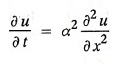…………(A)

when the steady state condition

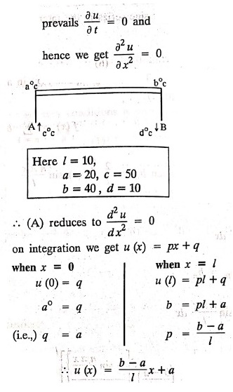
The boundary and initial conditions are

(i) u (0, t) = a for all t≥0

(ii) u (l, t) = b for all t≥0

(iii) u (x, 0) = f (x) = ((b –a)/ l) x+a for all x

Now, the suitable solution which satisfies our boundary conditions is given by

 u(x, t) = (A cospx + B sin px)        ……..(1)

Applying condition (i) in equation (1), we get

 u(0, t) = A  = a           ………..(2)

Applying condition (ii) in equ in equation (1), we get

u(0, t) = (A cos pl + B sin pl)  = b

…………(3)

From equation (2) and (3) it is not possible to find the constants A and B.

Since, we have infinite number of values for A and B. Therefore in this case, we split the solution u(x, t) into two parts.

 u(x, t) = u_s(x) + U_T(x, t)

…………. (4)

where u_s(x) is a solution of the equation  and is a function of x alone satisfying the conditions

 u_s(0) = c and u_s(l) = d

 u_T(x, t) is a transient solution satisfying equation (4) which decreases as t increases.

If u (x, t) is the subsequent temperature function the boundary and initial conditions are

(i) u (0, t) = c

(ii) u (l, t) = d

(iii) u (x, 0) = ((b –a)/ l) x+a

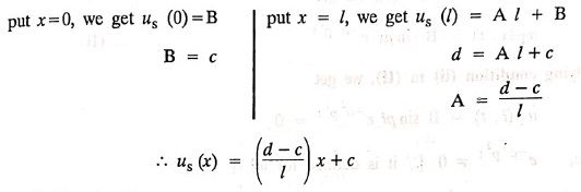
To find u_s (x)

u_s(x) = Ax + B

To find u_T (x, t)

4 ⇒

u(x, t) = u_s(x) + u_T(0, t)

u_T(x, t) = u(x, t) ‒ u_s(x)        ……….(5)

put x=0 in equation (5), we get

u_T(0, t) = u(0, t) ‒ u_s(0)

u_T(0, t) = c ‒ c = 0

put x=l in equation (5), we get

u_T(l, t) = u(l, t) ‒ u_s(l)

u_T(l, t) = d ‒ d = 0

put t=0 in equation (5), we get

u_T(x, 0) = u(x, 0) ‒ u_s(x)

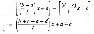
Given new boundary and initial conditions are

(i) u_T (0, t) = 0 for all t > 0

(ii) u_T (1, t) = 0 for all t> 0

 (iii) u_T (x, 0) = [ (b + c ‒ a ‒ d) / l ]x + a ‒ c

Now, the suitable solution is,

 u_T(x, t) = (A cospx + B sin px) 

      ……………(1)

Applying condition (i) in (1), we gets

 u_T(0, t) = A =0

Here,  ≠ 0        [it is defined for all t]

 A = 0

Substitute, A = 0 in equation (1), we get

 u(x,t) = B sin px   …….(2)

Applying condition (ii) in equation (2), we get

 u_T(l, t) = B sin pl  = 0

Here,  ≠ 0        [it is defined for all t]

B ≠ 0  [ suppose B = 0 already A = 0 then we get a trival solution]

  sin pl = 0

sin pl = sinnπ

         [sinnπ = 0]

 pl = nπ

Substitute, p=nπ/l in equation (2), we get

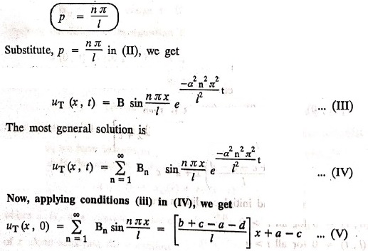
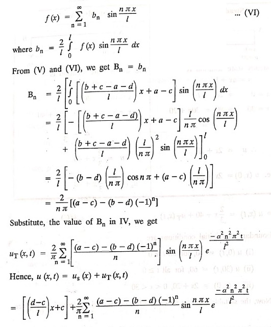
To find B_n we expand f (x) in a half range Fourier sine séries

Example 2: The ends A and B of a rod 30 cms long have their temperature kept at 20° C and the other at 80° C until steady state conditions 60° C prevail. The temperature of the end B is then suddenly reduced to 60° and kept so while the end A is raised to 40° C. Find the temperature distribution in the rod after time t.

Solution: The equation to be solved is 

…………..(A)

Here, there are two steady states

The solution may be u(x, t) = u_s(x) + u_T(x, t)

  ………….(B)

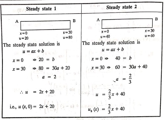
 (B) ⇒ u (x, t) = 2/3 x + 40 + u_T(x, t)

 ………….(C)

The boundary and initial conditions are

(i) u (0, 1) = 40, for all t≥0

(ii) u (30, t) = 60, for all t≥0

(iii) u (x, 0) = 2x + 20, 0 < x < 30

Now, the suitable solution which satisfies our boundary conditions is given by

 u(x, t) = 2/3 x + 40 + (A cos px + B sin px) 

   ………..(1)

Applying condition (i) in equation (1), we get

  40  = 40 + A 

A  = 0

 ≠ 0

          ['. it is defined for all t]

A=0

Substitute, A=0 in equation (1), we get

 u(x, t) = (2/3)x + 40+ B sin px 

       ………..(2)

Applying condition (ii) in equation (2), we get

  60 = 20 +40 + B sin (30p) 

   B sin (30 p)  = 0

  ≠ 0         [it is defined for all t]

 B ≠ 0         [. suppose B = 0, already A = 0 then we get a trivial solution]

 sin (30 p) = 0

sin (30p) = sin nπ

30p = nπ

p = nπ / 30

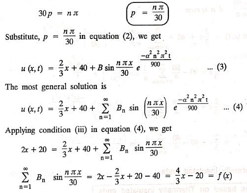
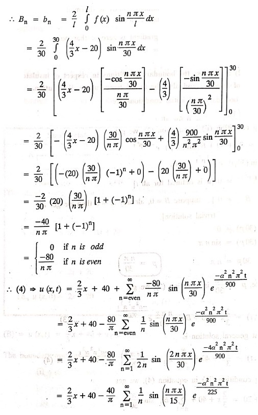
To find B_n:

Expand f(x) in a Half‒range Fourier sine series in the interval (0, l)