Fourier Series: One Dimensional Equation of Heat Conduction

ONE DIMENSIONAL EQUATION OF HEAT CONDUCTION

"Temperature ‒ gradient".

Consider a homogeneous bar of cross sectional area A. Take the origin O at one end of the bar and the positive x axis along the direction of heat flow. Let PQ be an element of length Δx and u(x, t), u(x + Δx, t) be the temperatures at time t at the ends P and Q respectively.

Then 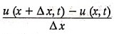 is the average rate of change of temperature with respect to distance in the element PQ.

The limiting value

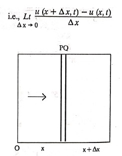
i.e., the potential derivative ∂u/∂x is the rate of change of temperature w.r.to distance, at p distant x from O. This is called the temperature gradient.

Example 1: What are the assumptions made while deriving one dimensional heat equation?

Solution:

We assume the following experimental laws.

1. Heat flows from higher to lower temperature.

2. The amount of heat required to produce a given temperature change in a body is proportional to the mass of the body and to the temperature change. This constant of proportionality is known as the specific heat of the conducting material.

3. The rate at which heat flows across any area is proportional to the area and to the temperature gradient normal to the curve. This constant of proportionality is known as the thermal conductivity (k) of the material.

It is known as Fourier's law of heat conduction.

Example 2: State Fourier's law of heat conduction.

The rate at which heat flows across any area is proportional to the area and to the temperature gradient normal to the curve. This constant of proportionality is known as the thermal conductivity (k) of the material.

It is known as Fourier's law of heat conduction.

Let R₁ be the rate at which heat enters the element PQ of the bar of cross sectional area A. Then R₁ = ‒kA (∂u/∂x)_x. This is mathematical form of Fourier's law. We put a negative sign, as (∂u/∂x) is negative. Heat flows from higher to lower temperature. As x increases, u decreases.

Note: The rate at which heat flows across any area is jointly proportional to the area and to the temperature gradient normal to the area.

Example 3: Write the p.d.e. of the one dimensional heat flow.

Solution:

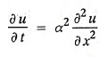
Example 4: The p.d.e. of one dimensional heat equation is  what is a² ?

Solution: α² is called the diffusivity of the material of the body through which heat flows. If ρ be the density, c the specific heat and k thermal conductivity of the material, we have the relation k/сρ = α².

Example 5: Explain why α² (instead of α) is used in the heat equation .

Solution: a² =  k/cp = positive

Since, the constants k, c, p are all positive

Hence, k/cp is denoted by α² (and not by α)

ONE DIMENSIONAL HEAT FLOW

We assume the following experimental laws to get the one dimensional heat flow equation.

1. Heat flows from higher to lower temperature.

2. The amount of heat required to produce a given temperature change in a body is proportional to the mass of the body and to the temperature change. This constant of proportionality is known as the specific heat of the conducting material.

3. The rate at which heat flows across any area is proportional to the area lo and to the temperature gradient normal to the curve. This constant of proportionality is known as the thermal conductivity (k) of the material.

It is known as Fourier's law of heat conduction.

Let us consider a homogeneous bar of uniform cross sectional area A.

Assume that the sides of the bar are insulated so that the stream lines of heat flow are all parallel and perpendicular to the area.

Take an end of the bar as the origin and the direction of heat flow as the positive x‒axis.

Let c be the specific heat and k the thermal conductivity of the material.

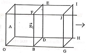
Consider an element got between two parallel sections.

BDEF and GHIJ at distances x and x + dx from the origin O, the sections being perpendicular to the x‒axis.

The mass of the element = Aρ δx

Let u(x, t) be the temperature at a distance x at time t.

By the second law,

the rate of increase of heat in the element = Αρδxc (∂u/∂t)

If R₁ and R₂ are respectively the rates of inflow, and outflow, for the sections x = x and x = x + δx, then

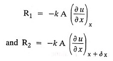
the negative sign being due to the fact that heat flows from higher to lower temperature.

i.e., ∂u/∂x is negative.

Equating the rate of increase of heat from the two empirical laws,

 Αρcδ x (∂u/∂t) = R₁ ‒ R₂

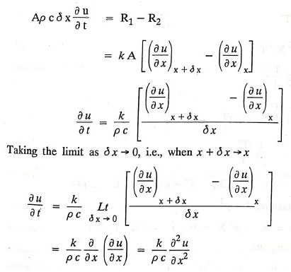
 k/ρc is called the diffusivity (cm²/sec) of the substance.

If we denote it by α², the above equation takes the form

SOLUTION OF HEAT EQUATION

The heat equation is

.......... (1)

Here, u is a function of x and t.

So, assume that solution of (1) is of the form

  u = XT         …….(2)

X is a function of x alone and T is a function of 't' alone.

 u = XT

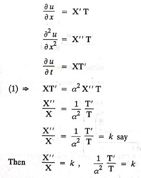
X" ‒ kX = 0        ……..(3)

 T'ka²T = 0... (4)

Case (i) Let k be positive k = p²

 (3) & (4) ⇒ X'' − p²X = 0 ; T′ – p²α²T = 0

The auxiliary equations are

m² ‒ p² = 0

m = ±p

m ‒ p²α² = 0

m=p²a²

we get X = A₁ e^Px + А₂e‒^px, T = A₃ e^P2a2t

 u(x, t) = ( A₁e^Px + А₂e^‒px) (A₃ e^P2a2t)

Case (ii) Let k be negative say k = ‒p²

Then (3) & (4), we get

 X'' + p²X = 0 ; T' + a²p²T = 0

The A.E are m² + p² = 0

m = ±pi

m + α²p² = 0

m = ‒a²p²

we get

X = A₄ cos px + A₅ sin px

 T = A₆ e^‒a2P2t

u (x, t)= (A₄ cos px + A₅ sin px)(A₆ e^‒a2P2t)

Case (iii) Let k = 0

Then (3) & (4) ⇒

X" = 0 and T' = 0

The A.E are m² = 0; m = 0

X = A₇x+ A₈; T = A₉

u (x, t) = (A₇x+ A₈) (A₉)

Thus the various possible solutions of the heat equation (1) are

(i) u(x,t) = ( A₁e^Px + А₂e^‒px) (A₃ )

(ii) u(x,t) = (A₄ cos px + A₅ sin px)(A₆ )

(iii) u(x, t) = (A₇x+ A₈) (A₉)

Example 6: How many boundary conditions are required to solve .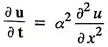

Solution: Three.

Example 7: State one dimensional heat equation with the initial and boundary conditions.

Solution: The one dimensional heat equation is

where u (x, t) is the temperature at time t at a point of distance x from the left end of the rod.

The boundary conditions are

(i) u (0,t) = k₁°C for all t ≥ 0

(ii) u (l,t) = k₂° C for all t ≥ 0

 (l being the length of the one dimensional rod)

The initial condition is

(iii) u(x, 0) = f(x), 0<x<l